Using a Raspberry Pi and INDI for astrophotography

I kind of stumbled into setting up a DIY astro cam through several earlier articles, and learning some ins and outs of the telescopes and cameras along the way. By the end of those articles I wasn’t entirely pleased with the results I got so I felt the urge to dig deeper. I started my adventures by writing a simple bash script and using tools such as libcamera-still to capture the RAW files and ssh to copy over the pictures, but this was not performing good at all so this felt like an interesting thing to improve. So I started to explore some options here.

Pre-setup

Make sure that you have a Raspberry Pi with Raspbian OS setup. In my case it’s a RPI2 with Raspbian 12 (bookworm). Also make sure to have SSH access and the disc space expanded to the entire sd-card space. You should also hookup the camera to the RPI:

And install the correct device tree overlay for your camera. In my case I had to edit the boot config and set:

#Camera
dtoverlay=imx462,clock-frequency=74250000

The libcamera library and userspace demo applications like libcamera-still, libcamera-vid and so on should already come pre-installed.

libcamera, libcamera-apps, rpicam-apps, pycamera2

Until now I’ve been testing with the utilities that come with Raspbian OS, being libcamera-still and friends. But what er all of these software packages exactly?

libcamera: a modern C++ library that abstracts the usage of cameras and ISPs away to make application development easier and with less gory camera specifics. Libcamera is developed as an independent open-source project for linux and Android.
libcamera-apps: a bunch of userspace applications that are build upon libcamera. It allows users to easily snap pictures, RAWs and videos using image sensors and ISPs that are supported through libcamera. It’s developed by the Raspberry Pi Foundation, therfor the libcamera library and libcamera-apps are developed by 2 different entities. More recently the apps/tools have been renamed to rpicam-apps to elaborate that the userspace apps and libcamera are 2 different things being supported by different teams.
rpicam-apps: previously named libcamera-apps, as you could read in the above
pycamera2: python library to make applications using libcamera as backend. It replaces the pycamera library that was created on top of the legacy Raspbian camera stack. As a python library it’s for many people a more convenient way to start hacking vision apps compared to directly using libcamera in a C++ project. Picamera2 also comes with a nice manual to get you going.

I started experimenting with pycamera2 myself a bit, but since I wanted a network solution I also started to think what other stuff I would need to develop. A REST based API? Maybe something with websocket for fast response? And how does that work in bad network conditions? Or could I maybe sail on the work of others? Well… meet INDI.

INDI

To quote their own words:

INDI Library is an open source software to control astronomical equipment. It is based on the Instrument Neutral Distributed Interface (INDI) protocol and acts as a bridge between software clients and hardware devices. Since it is network transparent, it enables you to communicate with your equipment transparently over any network without requiring any 3rd party software. It is simple enough to control a single backyard telescope, and powerful enough to control state of the art observatories across multiple locations.

INDI serves offers the networked approach that I’ve been achieving so by calling my libcamera commands over SSH, and it also has libcamera support so it fits my goal perfectly! But INDI is also a broad collection of many other software pieces coming together, not only for our Raspberry Pi based cameras but for many other cameras, controllers, motorized mounts and so forth. But let’s try to focus on some of the components that are of most interest for us.

indi, indi-libcamera, indi-pylibcamera, indi-3rdparty

indi: the core library
indi-3rdparty: a collection of all sorts of specific driver implementations for INDI.
indi-libcamera: this is just the specific 3rd party INDI driver for devices that are supported by libcamera. It’s basically just one of the many drivers in indi-3rdparty.
indi-pylibcamera: developed as an alternative driver implementation for indi-libcamera. However in contrary to the latter indi-pylibcamera is not part of the indi-3rdparty repository and probable will never be

I started by going through many pages of developer ramblings at the indib forum. From that Indi-pylibcamera seems to have matured best over the years and the author is very willing to help out with any issues that you have. But given it’s a alternative to the more official 3rd-party drivers repository I’m hesitating if it’s the best choice in the long run. The other way around the indi-libcamera driver doesn’t seem to be well maintained but I was willing to give a helping hand in case it was required. So let’s get started.

Compiling from INDI from source on Raspbian 12 (bookworm)

You can off course try to apt install all key components, but in my case I would end up with slightly outdated software and with libcamera support you mostly want the latest and greatest. Furthermore if I would be willing to help out with the development or debugging I’ll need to compile from source anyway. So let’s get our hands dirty…

To get the latest working software I’ll be building both indi and indi-libcamera from source, but also libXISF which is a dependency for indi that provides XISF support. But let us first install some build dependencies:

sudo apt-get install -y \
  git \
  cdbs \
  dkms \
  cmake \
  fxload \
  libev-dev \
  libgps-dev \
  libgsl-dev \
  libraw-dev \
  libusb-dev \
  zlib1g-dev \
  libftdi-dev \
  libjpeg-dev \
  libkrb5-dev \
  libnova-dev \
  libtiff-dev \
  libfftw3-dev \
  librtlsdr-dev \
  libcfitsio-dev \
  libgphoto2-dev \
  build-essential \
  libusb-1.0-0-dev \
  libdc1394-dev \
  libboost-dev 
  libboost-regex-dev \
  libcurl4-gnutls-dev \
  libtheora-dev \
  liblimesuite-dev \
  libftdi1-dev \
  libavcodec-dev \
  libavdevice-dev \
  libboost-program-options1.74-dev

Next we’ll be setting up a working folder:

mkdir -p ~/Projects

Let’s start with building and installing libXISF:

cd ~/Projects
git clone https://gitea.nouspiro.space/nou/libXISF.git
cd libXISF
cmake -B build -S .
cmake --build build --parallel
sudo cmake --install build

Next is indi:

cd ~/Projects
git clone https://github.com/indilib/indi.git
cd indi
mkdir build
cd build
cmake -DCMAKE_INSTALL_PREFIX=/usr -DCMAKE_BUILD_TYPE=Debug ~/Projects/indi
make -j4
sudo make install

Grab a coffee or somethings, this one is going to take a while if you’re like me building it on your RPI. Once done we can check if our indiserver is available with the latest version:

$ indiserver -h
2024-02-01T20:40:10: startup: indiserver -h
Usage: indiserver [options] driver [driver ...]
Purpose: server for local and remote INDI drivers
INDI Library: 2.0.6
Code v2.0.6. Protocol 1.7.

Now let’s continue with indi-libcamera:

cd ~/Projects
git clone https://github.com/indilib/indi-3rdparty
cd indi-3rdparty
mkdir -p build/indi-libcamera
cd build/indi-libcamera
cmake -DCMAKE_INSTALL_PREFIX=/usr -DCMAKE_BUILD_TYPE=Debug ~/Projects/indi-3rdparty/indi-libcamera
make -j4
sudo make install

With all of that set and done we’re on to the next step: using our new tools:

Starting the indi server

To be able to connect our host pc to the Raspberry Pi we need to run a indi server on the Pi. We can do so as following:

$ indiserver -v indi_libcamera_ccd

In the output you’ll notice the libcamera driver at work:

2024-02-01T20:54:29: startup: indiserver -v indi_libcamera_ccd
2024-02-01T20:54:29: Driver indi_libcamera_ccd: pid=5997 rfd=6 wfd=6 efd=7
2024-02-01T20:54:29: listening to port 7624 on fd 5
2024-02-01T20:54:29: Local server: listening on local domain at: @/tmp/indiserver
2024-02-01T20:54:30: Driver indi_libcamera_ccd: [3:09:59.402123462] [5997]  INFO Camera camera_manager.cpp:284 libcamera v0.1.0+118-563cd78e
2024-02-01T20:54:30: Driver indi_libcamera_ccd: [3:09:59.593527216] [6003]  WARN RPiSdn sdn.cpp:39 Using legacy SDN tuning - please consider moving SDN inside rpi.denoise
2024-02-01T20:54:30: Driver indi_libcamera_ccd: [3:09:59.604231695] [6003]  INFO RPI vc4.cpp:444 Registered camera /base/soc/i2c0mux/i2c@1/imx290@1a to Unicam device /dev/media1 and ISP device /dev/media0
2024-02-01T20:54:30: Driver indi_libcamera_ccd: [3:09:59.604426747] [6003]  INFO RPI pipeline_base.cpp:1142 Using configuration file '/usr/share/libcamera/pipeline/rpi/vc4/rpi_apps.yaml'
2024-02-01T20:54:30: Driver indi_libcamera_ccd: snooping on Telescope Simulator.EQUATORIAL_EOD_COORD
2024-02-01T20:54:30: Driver indi_libcamera_ccd: snooping on Telescope Simulator.EQUATORIAL_COORD
2024-02-01T20:54:30: Driver indi_libcamera_ccd: snooping on Telescope Simulator.TELESCOPE_INFO
2024-02-01T20:54:30: Driver indi_libcamera_ccd: snooping on Telescope Simulator.GEOGRAPHIC_COORD
2024-02-01T20:54:30: Driver indi_libcamera_ccd: snooping on Telescope Simulator.TELESCOPE_PIER_SIDE
2024-02-01T20:54:30: Driver indi_libcamera_ccd: snooping on Rotator Simulator.ABS_ROTATOR_ANGLE
2024-02-01T20:54:30: Driver indi_libcamera_ccd: snooping on Focuser Simulator.ABS_FOCUS_POSITION
2024-02-01T20:54:30: Driver indi_libcamera_ccd: snooping on Focuser Simulator.FOCUS_TEMPERATURE
2024-02-01T20:54:30: Driver indi_libcamera_ccd: snooping on CCD Simulator.FILTER_SLOT
2024-02-01T20:54:30: Driver indi_libcamera_ccd: snooping on CCD Simulator.FILTER_NAME
2024-02-01T20:54:30: Driver indi_libcamera_ccd: snooping on SQM.SKY_QUALITY

Kstars / Ekos client

On your desktop PC you have various indi clients available. I gave Ekos a try. Ekos is a cross-platform client. Open the KStars application:

You can start the Ekos utility by pressing Ctrl + k, or by navigating through the menu via Tools > Ekos. Next a wizard will be started to help you setup your observatory:

Select Next, and on the next step select the remote device option:

In the next window choose Other:

Now enter the IP address of our Raspberry Pi and click Next. PS: I also deselected the Web Manager option here, but more on that later.

And finally enter a profile name and click “Create Profile & Select Devices”:

You’ll be ending up in the Profile Editor window. Make sure to open the dropdown box and select RPI Camera to link the libcamera CCD driver that we loaded to a CCD in Ekos. Press Save.

Ekos is now being started:

At first nothing is shown in Ekos because we haven’t connected to our gear yet. Press the green play button. If you still have your ssh connection open to your Pi from those earlier steps where you started the indi server you’ll now notice a new incoming client connection:

2024-02-01T21:26:21: Client 9: new arrival from 192.168.0.221:42300 - welcome!

A new window will pop-up:

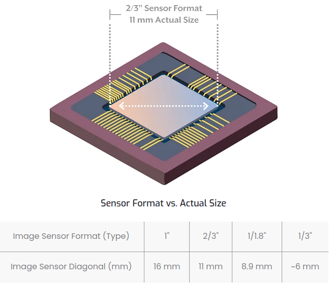
In the new window you can toggle the General Info tab to get some insights in the indi driver being at work. In my case it an IMX462 camera, but advertised as IMX290 since that’s how libcamera picks it up.

After pressing the Connect button you get a whole lot of camera settings that you can easily adjust through the GUI:

You may Close this window or minimize it, and once back in Ekos go to the CCD tab. Here you can start your first capture by pressing the camera icon below the sequence box, hovering the icon will tell you “Capture a preview”:

On the Raspberry Pi you’ll now see libcamera being set to work and capture that shot:

2024-02-01T21:51:00: Driver indi_libcamera_ccd: [4:06:30.151699548] [6070]  INFO Camera camera_manager.cpp:284 libcamera v0.1.0+118-563cd78e
2024-02-01T21:51:01: Driver indi_libcamera_ccd: [4:06:30.302132539] [6075]  WARN RPiSdn sdn.cpp:39 Using legacy SDN tuning - please consider moving SDN inside rpi.denoise
2024-02-01T21:51:01: Driver indi_libcamera_ccd: [4:06:30.307911048] [6075]  INFO RPI vc4.cpp:444 Registered camera /base/soc/i2c0mux/i2c@1/imx290@1a to Unicam device /dev/media1 and ISP device /dev/media0
2024-02-01T21:51:01: Driver indi_libcamera_ccd: [4:06:30.308089276] [6075]  INFO RPI pipeline_base.cpp:1142 Using configuration file '/usr/share/libcamera/pipeline/rpi/vc4/rpi_apps.yaml'
2024-02-01T21:51:01: Driver indi_libcamera_ccd: Mode selection for 1944:1097:12:P
2024-02-01T21:51:01: Driver indi_libcamera_ccd:     SRGGB10_CSI2P,1280x720/0 - Score: 3084.13
2024-02-01T21:51:01: Driver indi_libcamera_ccd:     SRGGB10_CSI2P,1920x1080/0 - Score: 1084.13
2024-02-01T21:51:01: Driver indi_libcamera_ccd:     SRGGB12_CSI2P,1280x720/0 - Score: 2084.13
2024-02-01T21:51:01: Driver indi_libcamera_ccd:     SRGGB12_CSI2P,1920x1080/0 - Score: 84.127
2024-02-01T21:51:01: Driver indi_libcamera_ccd: Stream configuration adjusted
2024-02-01T21:51:01: Driver indi_libcamera_ccd: [4:06:30.313121278] [6070]  INFO Camera camera.cpp:1183 configuring streams: (0) 1944x1097-YUV420 (1) 1920x1080-SRGGB12_CSI2P
2024-02-01T21:51:01: Driver indi_libcamera_ccd: [4:06:30.314471895] [6075]  INFO RPI vc4.cpp:608 Sensor: /base/soc/i2c0mux/i2c@1/imx290@1a - Selected sensor format: 1920x1080-SRGGB12_1X12 - Selected unicam format: 1920x1080-pRCC
2024-02-01T21:51:08: Driver indi_libcamera_ccd: Bayer format is RGGB-12

And a preview window will pop-up showing you your first capture!

You can save the preview to FITS, JPEG or PNG on your host pc by pressing the green ‘download’ icon in the upper left corner. Now what’s left for you is to enjoy that first picture that you just have token. At least I hope you have something more interesting than me to capture…

Autostarting indi-server

Until now I’ve been running the indi-server from the shell over an SSH session. Not really the most user friendly approach once you’re in the field, right. But there is indi Web Manager to the rescue. Indi webmanager is python based web application that can start and stop the indi-server for you by means of a REST api call. In lay mens terms it means that you can have the indi-server started by visiting a http web page, sort of. So what’s the difference with starting it over SSH? Well, the indi web manager is supported by Ekos in that it can make the required web calls to setup the indi-server through the INDI web manager. It also allows you to control what drivers need to be loaded. So in other means its also a manager to configure the indi-server plugins. But I found some difficulties installing it, furthermore since my setup is not changing a lot I figured that I didn’t need a daemon controlling our indi-server daemon but could as well create a small systemd service file and be done with it. So let’s go for that option and start creating our own systemd service.

First create a service file:

sudo nano /etc/systemd/system/indiserver.service

And enter following content:

[Unit]
Description=INDI server
After=multi-user.target

[Service]
Type=idle
User=pi
ExecStart=indiserver -v indi_libcamera_ccd
Restart=always
RestartSec=5

[Install]
WantedBy=multi-user.target

You must set the correct permissions:

sudo chmod 644 /etc/systemd/system/indiserver.service

Now you must reload the daemon lists so that systemd picks up the new service. Only then will you be able to ‘enable’ the service for starting with the OS:

sudo systemctl enable indiserver.service

The system will tell you that a symlink has been created.

sudo reboot

Reboot the system and the indi-server should come up after the reboot. If you’re still experiencing issues you can manually start the service using:

sudo systemctl enable indiserver.service

Next check the status of the service:

sudo systemctl enable indiserver.service

It should tell you that the service is active and running:

Press ‘q’ to quit. You can also inspect the service logs using journalctl:

journalctl -u indiserver.service

Example output:

Feb 02 22:29:34 rpi2 systemd[1]: Started indiserver.service - INDI server.
Feb 02 22:29:34 rpi2 indiserver[8617]: 2024-02-02T21:29:34: startup: indiserver -v indi_libcamera_ccd
Feb 02 22:29:34 rpi2 indiserver[8617]: 2024-02-02T21:29:34: Driver indi_libcamera_ccd: pid=8618 rfd=6 wfd=6 efd=7
Feb 02 22:29:34 rpi2 indiserver[8617]: 2024-02-02T21:29:34: listening to port 7624 on fd 5
Feb 02 22:29:34 rpi2 indiserver[8617]: 2024-02-02T21:29:34: Local server: listening on local domain at: @/tmp/indiserver
Feb 02 22:29:34 rpi2 indiserver[8617]: 2024-02-02T21:29:34: Driver indi_libcamera_ccd: [27:45:03.883924469] [8618]  INFO Camera camera_manager.cpp:284 libcamera v0.1.0+118-563cd78e
Feb 02 22:29:34 rpi2 indiserver[8617]: 2024-02-02T21:29:34: Driver indi_libcamera_ccd: [27:45:04.001222194] [8623]  WARN RPiSdn sdn.cpp:39 Using legacy SDN tuning - please consider movi>
Feb 02 22:29:34 rpi2 indiserver[8617]: 2024-02-02T21:29:34: Driver indi_libcamera_ccd: [27:45:04.006897368] [8623]  INFO RPI vc4.cpp:444 Registered camera /base/soc/i2c0mux/i2c@1/imx290>
Feb 02 22:29:34 rpi2 indiserver[8617]: 2024-02-02T21:29:34: Driver indi_libcamera_ccd: [27:45:04.007352574] [8623]  INFO RPI pipeline_base.cpp:1142 Using configuration file '/usr/share/>
Feb 02 22:29:34 rpi2 indiserver[8617]: 2024-02-02T21:29:34: Driver indi_libcamera_ccd: snooping on Telescope Simulator.EQUATORIAL_EOD_COORD
Feb 02 22:29:34 rpi2 indiserver[8617]: 2024-02-02T21:29:34: Driver indi_libcamera_ccd: snooping on Telescope Simulator.EQUATORIAL_COORD
Feb 02 22:29:34 rpi2 indiserver[8617]: 2024-02-02T21:29:34: Driver indi_libcamera_ccd: snooping on Telescope Simulator.TELESCOPE_INFO
Feb 02 22:29:34 rpi2 indiserver[8617]: 2024-02-02T21:29:34: Driver indi_libcamera_ccd: snooping on Telescope Simulator.GEOGRAPHIC_COORD
Feb 02 22:29:34 rpi2 indiserver[8617]: 2024-02-02T21:29:34: Driver indi_libcamera_ccd: snooping on Telescope Simulator.TELESCOPE_PIER_SIDE
Feb 02 22:29:34 rpi2 indiserver[8617]: 2024-02-02T21:29:34: Driver indi_libcamera_ccd: snooping on Rotator Simulator.ABS_ROTATOR_ANGLE
Feb 02 22:29:34 rpi2 indiserver[8617]: 2024-02-02T21:29:34: Driver indi_libcamera_ccd: snooping on Focuser Simulator.ABS_FOCUS_POSITION
Feb 02 22:29:34 rpi2 indiserver[8617]: 2024-02-02T21:29:34: Driver indi_libcamera_ccd: snooping on Focuser Simulator.FOCUS_TEMPERATURE
Feb 02 22:29:34 rpi2 indiserver[8617]: 2024-02-02T21:29:34: Driver indi_libcamera_ccd: snooping on CCD Simulator.FILTER_SLOT
Feb 02 22:29:34 rpi2 indiserver[8617]: 2024-02-02T21:29:34: Driver indi_libcamera_ccd: snooping on CCD Simulator.FILTER_NAME
Feb 02 22:29:34 rpi2 indiserver[8617]: 2024-02-02T21:29:34: Driver indi_libcamera_ccd: snooping on SQM.SKY_QUALITY

Again press ‘q’ to quit.

Other options within Ekos

Ekos and Kstart in general offers lot’s of possibilities, much more than I could ever come up with let alone implement them within any reasonable time. You can adjust exposure, set filters, adjust the format, and so on here:

You can also choose were to store the captured file: remote vs local:

And even create sequences with various exposures:

The the button next to the loop icon (which may have it’s icon missing due to a bug) is the one to start a video stream. You can even start recording the video from there:

Stability

I’ve been having some issue with DMA buffers no longer being able to allocate and so on. It always works the first time, but for a second picture or video I end up in trouble and need to reboot the gateway or manually restart the indi-server. So maybe it’s time to bump the libcamera version as well. Currently the Raspbian 12 (bookworm) OS comes with a slightly outdated libcamera v0.0.5 released back in the summer of 2023:

$ sudo apt show libcamera0
Package: libcamera0
Version: 0~git20230720+bde9b04f-1

We can update that to version 1.0.0 nowadays if we start from the official Raspberry Pi repo and compile from source. Before we get building we first need to install some more build dependencies:

sudo apt-get install meson
sudo apt install python3-jinja2 python3-yaml python3-ply

Now build:

git clonegit@github.com:raspberrypi/libcamera.git
cd libcamera
meson setup build
ninja -C build install

This will take again a considerable amount of time to complete, but if all went well we now have the updated libcamera installed:

pi@rpi2:~/Projects/libcamera $ libcamera-hello --version
rpicam-apps build: f74361ee6a56 23-11-2023 (17:01:08)
libcamera build: v0.1.0+118-563cd78e

Unfortunately that didn’t improve anything so I’ll be spending some time to see if we can debug things, but that’s for later.

Processing speed

This was one of the issues I had with my custom SSH script implementation that I wanted to speedup enormously. I was a bit hoping that having everything updated and moving over to a Raspberry Pi 2 would make drastic changes, like maybe 2 or 3 seconds at max for a 1 second exposure shot. I ended up finishing the 1s capture in 8 seconds. But for the 10s shutter I would again end up in over a minute easily. So it’s still far away from what I really wanted! So maybe not needing to open and close the application each time shoves off some time and also moving from a Raspberry Pi 1 to a RPI2 helps a tiny bit here and there, but unfortunately not what I had hoped. So I’m going to have to dive deeper into this matter and get why it’s so slow, do we really have that many parallel things going on here? More and that maybe in a follow up article if I find the time.

The verdict

I’m pleased with the result as all together I didn’t had that much difficulties to set things up. Except maybe for solving one missing build dependency, but that was pretty much it. I’ve had a lot worse build-from-source experiences in the past with other repositories! To my surprise the libcamera implementation is working OK, but the entire libcamera + INDI stack is not yet entirely bug-free. It’s also not yet as fast as I would have hoped for. That’s certainly something I’ll need to further dig into and check with the indi-3rd party team what could be wrong here.

The nice thing about all of this is that now I’m no longer on my own putting things together from scratch. I must say that it’s always fun to just hack yourself something together with a few lines of scripting, but at one point you’re going to have to make the trade-off of doing everything yourselves and spending a lot of time on it versus leveraging on other mens work and making a few mayor leaps forward. With INDI there is now the entire eco-system that’s readily at my hands and I can start exploring maybe adding a motorized mount, or maybe lookout for other desktop clients or maybe even mobile clients so that I don’t have to drag the laptop outside each time. Plenty of options and opportunities now fall within reach thanks to INDI and the open-source community! So I hope to have gotten you inspired to try things for yourself, and leave a line about how you’re experiencing the INDI, libcamera and RPI combination for your astro stuff. Good luck building!

Astrophotography from a beginners perspective, part 3: achievements

This is part 3 of my personal dive into astro photography. In part 1 we explored various telescopes types and in part 2 learned us the basics understanding of what makes an image sensor up for a certain type of job. In this part we’ll look into some of the result I obtained by putting all of that theory into practice.

Telescope of choice

Part 1 covered how I got to the Sky-Watcher Classic 150P telescope.

This telescope has a 150mm/6 inch aperture and a 1200mm focal length. Maximum magnification is x300. The actual level of magnification depends on your eyepiece, remember that we could calculate this as following:

magnification power = telescope focal length / eyepiece focal length

I have 3 eyepieces that I can use:

25mm: x48 magnification
10mm: x120 magnification
svbony 6mm: x200 magnification (purchased afterwards)

Camera

In my first astro shots I’ll be using my smart phone, a Samsung Galaxy S20 FE, as camera. It won’t give the best results but it comes free as I already own the device. Here are some specs:

Primary/main camera:

Sony Exmor RS IMX555
12MP
sensor size:: 1/1.76″
1.8μm pixels
f/1.8 aperture lens
focal length: 26mm
Night Mode
30x Space Zoom
field-of-view: 79°

Ultra-wide camera:

12MP
sensor size:: 1/1.3″
1.12μm pixels
f/2.2 aperture lens
focal length: 13mm
field-of-view: 123°

Telelens camera

8MP
sensor size:: 1/4.4″
1.0μm pixels
f/2.4 aperture lens : 3x optical zoom
focal length: 76mm
field-of-view: 32°

Front camera

32MP
4×4 pixel binning
field-of-view: 80°

The exact camera sensors weren’t officially revealed by Samsung but from searching around we found a source claiming that at least for the main camera the Sony Exmor RS IMX555 is used. While obviously not the best candidate for astro photography it’s still quite a decent sensor for every day use and even late evening shots. I couldn’t however find any extra info on that image sensor.

First shot

The results of my very first shots through this telescope using the Samsung Galaxy S20 FE were however not very great (given I took them holding the cam by hand) but at least promising enough for better to come. Here is that shot:

Sky-Watcher Classic 150P – 10mm eyepiece – x120 magnifying – Samsung Galaxy S20 FE

Using a smart phone adapter

Given the improved quality of smart phone camera we’ve seen special smart phone holders that allow you to mount your smart phone onto the telescope’s eyepiece so that you can get a steady shot. You can find them very cheap and therefor made them a no-brainer for me to try out.

Here is a picture that I made of our moon during daylight:

While not utterly sharp there are some nice details to see here such as the prominent Tycho crater near the top of the picture. Underneath is another one that made, several months later:

Sky-Watcher Classic 150P – 6mm eyepiece – x200 magnifying – Samsung Galaxy S20 FE

After that the weather turned bad and I had to wait a couple of weeks before I had some time again to sit out at night. This time Jupiter as on my radar. Here are some animated gifs I generated from videos that I’ve shot of Jupiter and 4 of its moons. The videos have been cropped and therefor enlarged a bit, reduced in length and some other tweaks applied to make the animated gif acceptable in size.

The first gif is from the first video that I made in standard video mode of the Samsung camera app. You can see Jupiter and 4 of its moons. From left to right: Callisto, Ganymede, Europa, Jupiter, Io.

Jupiter unfortunately reflects too much light compared to the black background and the app its default settings couldn’t cope with that very well. But honestly also for the human eye Jupiter is a bit over saturated. Not like in the above animation though, if you look closely enough you can spot the cloud belts. Than I found out there is also a Pro mode available. The second video was also made using the Samsung camera app but now using this Professional video mode. This mode allows you to configure the ISO, ‘shutter speed’, focus, white balance and zoom level. I went for zoom level 3, ISO 100 and speed 1/30. The WB is A 4400K and focus was set manually to 8. From left to right: Ganymede, Europa, Jupiter, Io

The Pro mode works out pretty well. While on the smart phone screen Jupiter still looks pretty small, after editing it turned out as above which is pretty OK for the inexpensive setup that I’m using. The additional zoom of the Samsung smart phone makes Jupiter appear larger than I get to see it through the telescope. It also allows me to get a better view on those cloud belts that Jupiter is so famous for.

Here is picture I made using the Samsung camera app in Professional mode. Settings: ISO 50, shutter 1/45, and a bit of zoom (3 or 4). Left: Jupiter, right: Io.

I slightly bumped the zoom level on the smart phone to get to the above result. As you can see Jupiter appears bigger but I don’t have a feeling we’re getting more details. I’m not sure what kind of zoom the camera actually uses but I’m guessing it’s kind of a digital zoom. To give you some idea about the distance of this object…

I also gave the Night mode a try. It’s kind of a counterpart for Google’s astro mode. Unfortunately this mode has some issues with the fast moving pace of Jupiter across the view port. Astro mode works great for still images, which is far from what happens when you mount your smart phone on top of a telescope. Failed effort, but non the less something I wanted to share. Maybe this could have turned out better when I would have had a good equatorial mount to compensate for Earth’s rotation.

For me the Professional mode of Samsung Camera app that I used in the earlier picture worked out quite well and gave me better results than I first anticipated.

Next challenge: the stars

Here is a shot in Professional mode of the Pleiades. The stars look quite dim and we didn’t really collect enough light to make them stand out in the picture. This is already at ISO 3200 and 1/10s shutter. It’s far from the pictures you see from NASA!

Bumping the shutter speed immediately results in less sharp result as stars move fast across the view port. I also gave Google astro mode a try just to see if it could cope with the movement of the stars. Unfortunately (but not unexpectedly) it could not and the star trails are even larger here:

So I’m guessing that without an motorized EQ mount or/and a way more sensitive camera it’s not going to get much better than shooting ‘nearby’ terrestrial bodies such as the moon and planets.

Other issues

Another difficulty that I found is that pointing the telescope to a deep space objects is not a easy task when you have your smart phone hooked up. For the moon or brights planets such as Jupiter or Saturn you can easy get a very good indication using a well aligned seeker and the fine tuning the last few bits using the feedback on the smart phone screen, but for anything darker than that it’s tricky and sometimes even trial and error until you get a good shot of the target object. You no’re no longer observing directly through the telescope but only have the camera’s feedback, and cameras are mostly not sensitive enough to show even most of the stars at sub second exposure times: mostly the smart phone screen is showing nothing but its common GUI objects! This is why motorized GOTO mounts are so handy, once aligned you basically command the telescope to point to a given object in the sky and you’re good to go.

Low end off-the-shelve astro cams

Off-the-shelve astro cams would definitely be an upgrade compared to the Samsung Galaxy S20 FE’s IMX555. The low end astro cams are low in costs but I’m not entirely convinced if they’ll be that much more sensitive, it’s maybe not good enough to shoot deep-sky objects though the telescope using a low shutter time. Maybe the high-end cams can, but then again they’re not within my budget. One of such more affordable off-the-shelve astro cams is the Player One Mars-C Color camera which can be found for less then € 250 nowadays.

What about DIY?

Even though the price of the Mars-C is not out of this world, it’s still far from the budget I’d be willing to spend. In the end it’s just a very experimental hobby thing… So what’s available on the DIY market? Well the IoT market has been flooded with cheap CSI and USB cams that you can hook up to your favorite hacker board. The cams are dirty cheap but certainly not of best quality. In more recent years the Raspberry PI foundation has made some decent DIY cams available:

	Samsung Galaxy S20 FE	Raspberry Pi High Quality camera	Raspberry Pi Global Shutter camera	ArduCam SKU 2MP IMX462 (B0444)
sensor	Sony Exmor RS IMX555	Sony Exmor RS IMX477R	Sony Pregius IMX296LQR-C	Sony Starvis IMX462
sensor size	14.4mm (1/1.76″)	7.9mm (1/2.3″)	6.3mm (1/2.9″)	6.46mm (1/2.8″)
resolution	12 MP	12.3 MP	1.58 MP	2 MP
pixel size	1.8μm	1.55μm	3.45μm	2.9μm
illumination	back	back	front	back
shutter	?	rolling	global	rolling
mono/color	color	color	color	color
application	consumer cameras	consumer cameras	embedded vision	security cameras

I’m not sure if this is a coincidence but all cameras here seems to be Sony branded. Sony Pregius sensors have been focused on embedded vision and therefor contain a global shutter and also perform quite well under low light conditions. The latest variant (4th generation) is the Pregius “S” which even features back-illuminated (BSI) CMOS. While the IMX296LQR-C does not yet contain that technology it still comes with pretty large pixels, hence why it also performs relatively good under low-light conditions. This is also the specific application that the RPI foundation had in mind. That aside there is also the Sony Starvis and more recently Starvis 2 series. Those sensors both come with BSI and also performs very well in near-infrared (NIR) light conditions which gives them a clear advantage over the traditional Pregius sensor in performing night-sky observations. The Starvis series are focused for usage in for example security camera applications but are also often found in astro cams. The recently introduced Starvis 2 features optimised pixel structures and therefor have a higher dynamic range and higher sensitivity than the previus Starvis generation. Sensors like the Sony Starvis 2 IMX585 are much sought after within the astro community. The Sony Exmor series has been evolving for more than a decade already. The Exmor series focuses on low noise high quality image sensor. Actually, the Starvis series are a subset of the Exmor R series (the fifth gen Exmor), where the R suffix stands for back-illuminated. Exmor R sensors have been build starting from 2008. Exmor RS is the next iteration of Exmor sensor which on top of BSI brings improved performance in the NIR spectrum due to the new Stacked image sensor technology. Hence the S suffix… Exmor RS was announced in 2012. While Exmor RS is great for wide range of applications but not specifically on one specific area, the Starvis series are optimized for the low-light conditions that security cameras often have to deal with.

For further details I recommend looking at following pages on the e-Con systems website who are specialists in computer vision:

I’ve been looking for easily available Starvis sensors on the internet. It seems that as far as consumers go the Starvis 2 series can not yet be found as board camera for dirty cheap. That’s why I added the slightly older IMX462 sensor in my comparison. It’s a 1st gen Starvis sensor that’s still relatively close to Starvis 2 series in performance. It has about 2.5x to 3x bigger pixels compared to the Samsung S20 FE camera which gives us a rough indication on how much more light falls into the sensor. It can for example be found in Player One Mars-C Color camera which was mentioned a bit earlier.

DIY test: Sony Starvis IMX462

On Amazon I found a camera board similar to the ArduCam IMX462, the Chinese made Innomaker CAM-MIPI462RAW. This board camera can be found for roughly € 30 which is cheap enough for my adventures.

Innomaker IMX462 sensor

The CAM-MIPI462RAW is advertised as Raspberry Pi camera and uses the CSI connector to hook into the RPI. It seems the IMX290 driver can be used to work with this camera board since it has matching registers. I hooked it up to an old Raspberry Pi 1B I had still laying around unused.

Edit the boot config (/boot/config.txt) as following:

#Camera
dtoverlay=imx462,clock-frequency=74250000

We can use libcamera to work with the image sensor, to see if the sensor has been probed:

$ libcamera-vid --list-cameras
Available cameras
-----------------
0 : imx290 [1920x1080] (/base/soc/i2c0mux/i2c@1/imx290@1a)
Modes: 'SRGGB10_CSI2P' : 1280x720 [60.00 fps - (320, 180)/1280x720 crop]
1920x1080 [60.00 fps - (0, 0)/1920x1080 crop]
'SRGGB12_CSI2P' : 1280x720 [60.00 fps - (320, 180)/1280x720 crop]
1920x1080 [60.00 fps - (0, 0)/1920x1080 crop]

We can then use libcamera-still to capture still images in .jpeg and .dng format. I made a few tests to see how the new sensor lines up to other sensors. During this test I kept the shutter speed at 1/10. Here is the command I used:

libcamera-still -n -o "pic.jpeg" --gain 0 --awbgains 0,0 --immediate --shutter=100000

First I took a shot using a IMX219 sensor. I haven’t addressed this sensor so far, but here as some specs: rolling shutter, 3280 x 2464 (8MP resolution), sensor format 1/4″, 1.12μm pixel size.

Roughly the same shot, same lighting, and same moment but now using the IMX462:

It’s remarkable how the IMX462 clearly shows a brighter result. A lot more detail are exposed in the dark. It’s no surprise given the IMX219 is of an entirely different sensor category. And while it theoretically outperforms the IMX462 in resolution as you understand by now it isn’t of much use in such low-light conditions.

I repeated that shot but now using my Samsung Galaxy S20 FE in Pro Camera mode, using that same 1/10 shutter speed and ISO 50.

Samsung Galaxy S20 FE in Pro Camera mode 1/10 shutter speed ISO 50

And again with ISO 400:

Samsung Galaxy S20 FE in Pro Camera mode 1/10 shutter speed ISO 400

So as you can see the IMX462 is a quit decent low light cam compared to some of the other solutions I have available. But as I also mentioned it may not be a big step forward compared to the more then decent IMX555 sensor found in the Samsung Galaxy S20 FE. Considering capturing Jupiter can already be scraped from the list, and I’m still not convinced the IMX462 is up to the task of deep space imaging, I guess we’re going to need more tricks to get any decent result out of this.

Astro software

An area that we haven’t thoroughly touched but certainly deserves more attention is software. One implementation that’s widely available and used is the astro feature found on Google and Samsung smartphone. While the implementations may differ slightly, the basis will overall mostly be the same. So what dark secrets have they coded in their camera? Well in fact Google is glad to explain a thing or two about their astrophotography implementation. I’d strongly encourage you to go through their 2019 article about Night Sight on Pixel Phones.

The idea: achieving long exposure shots by stacking multiple semi-long exposure shots together. Before you praise the smart guys at for their wonderful idea, the isn’t entirely new for the real astro guys. The image stacking technique has been used for years in advance before Google started to add it to their smartphone software. The technique avoids having to use very long exposure shots since anything more then about 15s will form trails. With sub 15s exposure times the stars will mostly remain still. If you take 15 of such pictures and stack them using software you’ll achieve a virtual exposure time of 150s which will show you more details of the night sky than you can see with the naked eye. The google software even allows to collect light for up to 4 minutes. The software will need to stack the different images together. However there is more than meets the eye here. Over the different images the stars will still have moved a bit in position due to the earth’s rotation, thus the stacking software needs to be able to exactly align all images. More trickier is that while the night sky moves across the lens throughout the night, foreground objects such as the landscape, houses and trees will not. That’s where the Night Sight mode on pixel phones really shines. It would be really neat if we could just plug in our own camera into our smart phone and let the software do its thing. Driver wise obviously this is not something we can expect at this moment. Image stacking also helps reducing noise. There is a lot of noise in images and they may become very visible when you’re shooting against a pitch dark sky. The guys at PetaPixel did a very short but clear article why image stacking helps reduce noise and recover signal. The importance of stacking is that you use different pictures stacked together and not the same picture, because in essence it’s those variations of noise that will get averages out and therefor improve image quality.

Here is an example I found on the internet of image stacking at work:

Just a quick mention along the way: Electronically Enhanced Astronomy (EAA) is a form of astronomy where the celestial objects are not observed through an eyepiece but instead indirectly by means of a camera and stacking software. Actually what we described in the above. Some in depth info can be found on the skiesandscopes.com website.

Now to the software itself… what’s the stuff to get? Spoiler alert: it’s not Photoshop! And that actually came a bit as a surprise. Well, off course you can, but dedicated astro tools focus on automating things that matter for astr shots. There are many different astro tools around that’s actually not so easy to decide on which one will work for you. Some are open-source and free, other’s are behind payment wall. Here is a small overview:

Name	Sharpcap	Firecapture	Siril	DeepSkyStacker	Open Astro Project	ASTAP
Description	Planetary, lunar, solar, deep sky and EAA. Stacking. Wide camera support.	Planetary capturing, broad astro cam support, feature full. No stacking	Editing, stacking, live stacking. Went past v1 status	Primarely focused on image stacking	Planetary imaging, development seems to have dried out	Stacking and plate solving for deep sky imaging. Feature full
Open source	no	no	yes	yes	yes	yes
Platforms	Windows 7 up to 11	Windows, Mac, linux	Windows, Mac, linux	Windows	MacOs, linux	Windows, MacOs, Linux
Price	normal: free pro: £ 12 / year	free	free	free	free	free

This is just a small fragment of the many tools out there. PixInsight, another tool worth mentioning could easily have been added here, but unfortunately comes with a fee of around € 350 (incl. VAT) which is out of my budget. From the above list my first filter is that I want native linux support. That already rules out half of the software out there. From the remaining list I got mostly charmed by Siril. The website is refreshingly new, and by watching a demo on YouTube it also seemed to me that image stacking was just a matter of toggling a few buttons. What I also find interesting is that it can do the stacking live as you drop pictures in the working folder. This sort of brings it closer to Google’s Astro mode for Pixel phones. Firecapture and ASTAP are two other solutions that are popular for linux systems. They’re both integrated in Astroberry.

Stacking video

Video stacking is another technique used to improve image quality, but I only discovered it 2 months after I first started typing the first words for this article. It’s kind of like image stacking, but now using a video as source of information. This works out pretty well and is sometimes preferred of image stacking. As some people explains it well on dpreview.com forums:

“What is the pros and cons of say stacking 5 mins of video of Saturn agains say lots of 5 second photos of Saturn stacked? I’ve never stacked before but just seen a video of someone who stacked a video rather than photos. Thanks .”

“Most planetary cams are shooting at 60-120 FPS. Multiply that by 5 minutes, and then have software that auto- detects the sharpness of each frame and only chooses the very best 5-10%.”

“Dave, you do not want to stack 5 sec pictures of saturn… ever. No way you will get a sharp picture that way. As described by swim, people use video, and ‘lucky’ imaging. The idea is to shoot many frames, 1000s, as in 30frames per second or higher After a few 2 minute videos, you hope you got lucky, and some of the frames are sharp. Atmospheric turbulence is the enemy, and shooting 1000s of frames, increases the odds that some frames were captured in a calmer part of the turbulence. The software analyzes the frames pics the best ones and makes the stack. Almost everyone is doing the planets, and close ups of the moon this way, I am hoping to try it myself, as soon as the planets are out at night. Most will recommend an astro camera, but I will try with my Canon 60D, or 7D mkii. Tons of good info out there, just google lucky imaging.”

The image below shows the atmospheric turbulence at work:

The two programs that you can use for recording video files are FireCapture and SharpCap. Make sure to avoid compressed video file formats.

Personally I’ll not be focusing on video stacking this time, but it’s certainly a technique worth mentioning and maybe I give it a try in the future so I wanted at least to mention it here so that you can start exploring by yourselves.

Live image stacking

So with Siril installed I got to perform my first tests. I made a shell script that eases the process of remote triggering libcamera to make raw images in .dng format and then secure copy them of the network to my host pc. I started Siril and set it up for live stacking, monitoring the output dir of my script.

-------------[pi@192.168.0.205]-----------------
1. single shot
2. interval shots
3. start camera stream
4. clean remote disk
5. setup camera
6. exit
Select option:

But I ran into a big bummer, the software wasn’t taking any of my pictures. So after spending the evening trying different image formats and sources I found out it was a bug in the Siril software. I filed a bug report but afterwards spend some time on fixing the issue myself and giving the solution back to the community. My first attempts at stacking where disastrous. While it seemed all that simple in the video, I couldn’t get very pleasing result out of it. Maybe it was the weather… it’s been poring rain for weeks so I was forced to test stacking on my interior, and on semi cloudy nights. Also the lens has quite a bit of barrel distortion which may confuse the aligning algorithm, more on that later. I tried off-line stacking by reading the docs but still couldn’t figure out how to get a decent output. Finally I set up the camera on a nearly clean lookout with nearly nothing else in the pictures as stars, and some slightly visible clouds. I but the RPI on a tripod this time:

Using interval shots I took 30 pictures of with each 10s exposure. I’m not sure how Siril thinks this makes total of 9 minutes cumulative exposure…

Here is how one of those 30 individual images looks like:

You can clearly spot the cloud on the picture here, but also some stars can be recognized.

And here is what came out of the stacking process:

So what we see is that slightly more stars are visible, and they also stand out it bit better. The clouds that slightly block our view on roughly all pictures are mostly gone, and also the space between the stars contains less noise. At the edges you notice a bit of star trails being formed because of the aligning process. I guess not correcting the lens distortion has that effect a bit. Also having parts of the house and trees in the picture is certainly not a good idea as they come out all washed out.

Lens (barrel) distortion

The camera lens is probable too wide for my application. The current lens has following specs: Fov(Diagonal)=148 degrees. Barrel distortion gets more and more noticeable when the Fov increases and in my case it’s very noticeable!

Compared to the Samsung Galaxy S20 FE this is even wider than what Samsung labels as their Ultra Wide Camera. Actually when we compare it to the main camera on the S20 FE which is closer to a 80° field of view I clearly made a mistake with this sens. It may be OK for close up shots in applicationq such as a smart doorbell, but I instead want to capture preferable smaller parts of the night sky so I may want to change to the field-of-view closer to something a telelens has to offer.

I’m not entirely sure the stacking process can cope well with this type of distortion. Barrel distortion can be corrected in software like Gimp, Photoshop, opencv and many more, or sometimes even through dedicated hardware DSP or ISP. As you understand in both cases careful tuning or calibration must be performed. Raspberry Pi’s don’t come with a hardware support for lens correction, doing the correction on the CPU is one option but it will take some time though. Furthermore you’ll also risk some loss in detail. One workaround could be to just go for a smaller angle lens. The Arducam IMX462 for example comes with Fov(H) of 92 degrees, or even go one step further into the realm of tele-lenses. The latter are however not widely available for the S-mount (also referred to as M12 mount) of my camera.

Capturing speed

Aside of that I still would have expected a better end result though. One other thing is that the RPI 1B is really slow on capturing images. A failed command takes already 5s. A 10ms exposure takes 7.5 seconds to capture. A 1s exposure takes already 14 seconds, and for a 10s exposure the camera takes already more than a whole minute. Therefor taking the batch of 30 images took about half an hour. Luckily this happens unattended. During the time span the stars have moven quite a bit already where ideally it should have took only a minute of 5. Keeping the time span smaller will also lower the effort in software on getting everything stacked properly. I did a small optimization by storing the images in RAM, but that was only a small bonus. Having a faster Raspberry Pi could help here, but also the usage of an hardware ISP can be useful to speed up the image processing. Both things I unfortunately don’t have. Some info about libcamera ISP integrations can be found here: https://starkfan007.github.io/Gsoc-summit-work.

image courtesy of jivp-eurasipjournals.springeropen.com

Many of the processing steps that the CPU performs in my case can also be performed by an ISP. The new Raspberry Pi 5 now performs part of the pipeline already and a small ISP like preprocessor based upon their RP1 chip.

Image courtesy of the Raspberry Pi Foundation

Foreground vs background

Furthermore, it would tremendously help if the stacking software was able to differentiate the foreground from the background. Things in the foreground don’t move at all and require different alignment than things in the back. It would help if we could tell the stacking software what part of the image requires star aligning, and what not. This is something the google AI is trained for pretty well and leads to very good end results. Using a tele-lens or telescope with narrow field of view will also help.

Camera tuning

As of my understanding we’re also relying on a libcamera tuning for the IMX290 which may slightly differ from the IMX462. The camera calibration process is documented quite well in the official Raspberry Pi Camera Guide, but will also take some money and even more time both of which I’m not willing to spend on it. Good camera calibration will lead to beter image quality.

Image noise

When I look at one of the original picture I fed into the stacking process I also notice quite a bit of noise. Here is that:

From the stacking end result we notice this gets filtered out pretty well. I’m still surprised we get this amount of noise that, I would have expected better results from a camera sensor that states to be “low noise high sensitivity”. Hardware design does play a role here. Sensors are sensitive to ripple on the power supply and a proper ripple filter could always helps to improve the image quality here. There is a small amount of filtering on the back of the sensor board though so I’m guessing there isn’t much use in trying to improve this area.

Cooling

Camera sensors are sensitive to light, and image quality improves once you start cooling the camera. You can already see an effect when you put the camera outside during freezing cold nights.

Image courtesy of player-one-astronomy.com

One way camera’s are often cooled is by using a Thermo Electric Cooler (TEC):

Image courtesy of Blaze2A at webastro.net

TECs come in various sizes and have a wide gamma of operating voltages and cooling power making them very applicable for cooling CMOS sensors. The downside however is that TECs by themselves are not very efficient compared to phase change cooling, the hot side of the TEC has to be cooled properly, dealing with both the sensor’s heat as the TEC’s heat. If one TEC does not suit your purpose you can also stack TECs, but know that the only makes the entire thing even harder to control. And then there is also moisture… Once you get below the dew point moisture is something that you need to take into account as condensation will form quite fast on various places in your camera body. Although I do have some electronics available and also TECs laying around unused, for now I’m going to try to avoid it since I’ll probable not be able to take very long exposure shots anyway. If you’re a DIY’er like me I can recommend following web pages:

Lens mountings

Lenses come it all sorts and sizes and same can be told about cameras. Hence there is no universal one-fits-it-all mounting that makes everything compatible. However, things have kind of standardised over the years and we now have mountings that are commonly used over different brands, making everything a bit more interchangeable. Here are a few well used mounting options that I need to take into account.

M12 (S-mount): this is the smallest lens mount option and therefor also the cheapest. This mounting option is commonly used on various camera boards and are particular interesting for webcam, security cams and such because the mounting and lenses are compact.

CS and C: roughly the same mounting but with different flange focal distange. Used with bigger and more high quality lenses.

1.25″: typically used on telescope lens mount. This is the one I’m going to need to adapt to when I’m going to fit the Raspberry Pi on my telescope

With that we now have an understanding of how we can fit the Pi camera onto the telescope: a M12 to 1.25″ adapter. We could print them ourselves, however the cost of it would almost always match those of the cheap adapters that you can find on Amazon. Along the way I also learned that the material of the adapter also plays an important role, you don’t want to go with material that’s too much reflective. So that’s another reason to go for off-the-shelve adapters. I specifically went for the EBTOOLS 1.25″ M12 x 0.5 T Ring Telescope Mount Adapter:

Camera board with M12 adapter fixed to Raspberry Pi:

Telescope mounted pics

Well we know the IMX462 is a bit more sensitive to light then the results I’ve obtained with the Samsung S20’s main camera, but non-the-less we’re not going to be performing long exposure shots on the telescope since the IMX462 is also not sensitive enough to capture stars and nebulas with fast shutter speeds. Due to the bad weather we’ve been having for month it took me a long time to finally go outside with the mounted IMX462. Finally on a cold winter night I had my first play with the new camera but due to the absence of the moon I directly gave Jupiter a shot.

Sky-Watcher Classic 150P – IMX462 – Jupiter

Auwch, that’s a horrible picture! I don’t know what went wrong here but I found it impossible to get the focus correct. In video mode it was as if Jupiter was on fire, with artifacts all over the place. Okay, I may lower the exposure here a bit, I agree, but optically things don’t really look that well.

After spending some time to check whether I can get any half decent out of the camera during daylight I went back to give astro shots another chance. This time the moon was up and it’s a far easier target to shoot as it requires only very small exposures.

Sky-Watcher Classic 150P – IMX462 – Moon – 1ms shutter, gain 0

Again, but I slightly tweaked the focus a bit more and also recorded in RAW format:

Okay, this is starting to look like something. Maybe not all that nice, the picture is still a bit unsharp even when I really gave it my best to get it focused well. There are also a lot of visual artifacts in that image, notice the horizontal lines in the bottom corner, especially in the first attempt. Here is another attempt at Jupiter:

Sky-Watcher Classic 150P – IMX462 – Jupiter – 1ms shutter, gain 0

You can clearly notice how the image is sharper than the first attempt. I also increased the shutter speed a bit to reduce the overexposed Jupiter surface. However adapting the shutter more than what I used in the above picture didn’t result in a better picture.

Next I gave the Orion Nebula (M42) a try. Now due to the focus not entirely correct it’s again all smudgy, but you can see the some contours already of the Nebula.

Sky-Watcher Classic 150P – IMX462 – M42 Orion Nebula – 500ms shutter, gain 20

500ms is really about the maximum I can set the shutter to before star trail artifacts become visible. In order to capture something of the nebula the gain had to be increased to 20 or above. There is a lot of visible horizontal banding noise (hbn) in this image, but we already saw those in the moon pictures too. The higher gain values however makes them stand out a bit more here.

I had only 2 pictures taken during that timeframe, but I tried to sack them anyway using Siril. I had to apply a severe translation to align them properly so maybe half of the image didn’t get stacked at all and I had to seriously crop the end-result. I also applied a de-noising and banding de-noising filter.

Sky-Watcher Classic 150P – IMX462 – M42 Orion Nebula – 500ms shutter, gain 20 – stacked, de-noised, cropped

Okay, it didn’t really improve the image quality that much, but some small gains are obtained non-the-less. For now I’m still not very impressed by the end-result, but I do feel like I’m still progressing.

What can we learn from off-the-shelve astro cams?

Companies such as ZWO, Svbony and Player One have been dominating the market of affordable off-the-shelve astro cameras for years now, so it be worth investigating what’s under the hood there. Only issue is that I don’t own such a device myself, so I had to search around on the internet f someone else who documented the process. What I noticed is that the camera sensors in use isn’t really top secret for those camera vendors. In contrary they seem to even highlights what sensor that they use, so that the customer with some technical background (which probable most have anyway) will have some food for comparison and understanding. Also the mechanical design is here and there mentioned, but I’m more looking into the hardware that they have in place. I’m assuming that they have a cost optimized but still low latency design in place, so it’s really interesting how that compares to the Raspberry Pi’s that are found in many hobbyist projects. I couldn’t get my hands on a step be step teardown, but fortunately I stumbled upon following picture of someone who did a cooling job on a Svbony sv705c camera with IMX585 camera.

Image courtesy of Stipe Vladova at cloudynights.com

The Winbond W631GG6NB-12 chip at the far right side is a 128 DDR3 RAM chip, nothing special there just some way of storing things fast along their way outside the camera. The 2 other chips are a bit harder to read what they’re labelled with, but at least from the one in the middle we can clearly see it’s labeled with Trion. This didn’t immediately ring a bell for me, but a quick google lookup brought me to the Efinix website. The Efinix Trion chips are actually FPGAs focussed for usage with MIPI CSI cams. They have a wide range of control interfaces (I2C, UART, SPI, …) and output interfaces (LCD, LED) and can directly interface with the Winbond DDR3 memory. From what I can read we have a Trion T35F324 chip here which currently sell on Digikey for prices between €20 and €30. Typically usage for these FPGA’s:

… so this is actually the very core of the camera here! It directly takes the Bayer data from the camera sensor and performs image processing upon it via it’s programmable ISP. The third chip, the one at the top, isn’t clearly captured in the shot we found on the internet. I’m assuming it’s some kind of interface chip to USB, or maybe micro controller manages the various settings and such and is in control of everything.

Another example, the ZWO ASI 224 MC uses a Lattice FPGA. The XP2 DVKM V1.2 mainboard (not the one in the picture below) hosts particularly a Lattice LFXP2 FPGA, a Toshibe TLP291-4 octo-coupler (nothing sexy there) and a Infineon CYUSB3014 SuperSpeed USB Controller with on-board ARM CPU.

Other brands are equally less open about their internals, where Svbony and ZWO are relying on an FPGA I’m quite sure each brand will have their own strategy on how to achieve good and speedy images. It’s assumable that the implementation will even vary depending on the model of camera, even within the same brand. In general, for which I also include non-astro, many flexible ISP solutions rely on FPGAs. For example you may also check out the solutions of helion-vision.com.

Other inspiring projects

I’m obviously not the only one to slab a Raspberry Pi to their telescope. I found several others who tried to give it a shot, but most of those projects date from few years back where the availability off retail CSI camera modules was less scars and the official RPi cams were not the greatest either for astro-photography. In more recent years some attempts have been made to utilize the RPI HQ Camera with better results.

https://terramex.neocities.org/astro/ : an image gallery of astro pics taking with the HQ cam. The guy clearly knows how to get great astro shots, the results are really amazing!
https://www.hackster.io/news/hubble-pi-is-a-raspberry-pi-based-astrophotography-camera-63f7c3b03a17 : small description of the Hubble-Pi project.
https://github.com/RemovedMoney326/Hubble-Pi : the sources of the previously mentioned Hubble-Pi
https://adambaskerville.github.io/tabs/astro/ : another hobbyist project running a GUI over VNC

Some of these projects as a solution run the GUI on the Pi itself either directly using an LCD or remotely via VNC. I didn’t want to go that way and keep it simple in such way that it’s just a bash script with little dependencies, you only need to have libcamera and ssh working. The network interface can be ethernet, or in my case Wifi (client mode). The script basically shoots the libcamera commands as if you would call them manually, but at the ease of selection menu options instead of typing it all out. After some time playing around I would say that maybe GUI application fits better here to control all little things at a click of the mouse instead of navigating through the cli menu. The ultimate solution would be if we could just shove it somehow into existing solutions so that we get features for free and remove or at least reduce maintenance.

Another very nice website to check out is:

https://landingfield.wordpress.com/ : builds his own low-light camera using an FPGA and DLSR camera sensors. Very recommended to check out, very tech savvy.

To quote one of his conclusions: ”FPGA still provides the flexibility that we want. And in some cases designing the data paths to suit mission requirements“

And you may also like this forum thread:

https://forum.radxa.com/t/connect-arducam-hq-camera-to-rock5b/12325 : Connect Arducam HQ Camera to ROCK5B
https://stargazerslounge.com/topic/399998-why-should-you-buy-dedicated-astronomy-camera-and-not-to-try-to-invent-your-own: Also tried to hook up the Sony IMX462 for astro purposes
https://github.com/aaronwmorris/indi-allsky: All-night camera software support many cameras (including RPI) through INDI

Conclusive thoughts

With reaching out those other projects for other to explore I feel like reaching the end of my 3-stage article on “Astrophotography from a beginners perspective”. During the several months that I was working on this project (mostly in late night evenings) I feel like having gained some beginners insights in astro-photography, but maybe also a little bit about photography as a whole. I don’t want advertise this 3-part introduction as the definitive guide though as I feel that some details may not be 100 percent accurate, but also that there is much more to explore and details to grasp. See it more as my personal journey through getting to know a bit about the ins and outs of taking nice night sky pictures.

If I need to take any conclusions than those would be the following:

For a first telescope a Dobsonian is good to start with if you only care about low exposure shots of the moon and maybe some planets.
For long exposure shots you definitely need a motorized EQ-mount. Dobsonian and alt-az mounts may also work but are more rare.
If you get any decent size telescope don’t cheap out on the mounting: if you can’t get a stable scope you won’t get to see any night sky objects either.
With telescopes, mostly the bigger, the better you’ll be able to capture deep-sky objects. But even sub-500 scopes should be good enough to show you something, and also give you some spectacular views on the moon and planets of our solar system.
There are several photo editing software for various OS. Try to experiment with some of these yourself and see what works for you.
There is a whole spectrum of image sensors out there. Sensors are build for various purposes, and thus only some of them will fit well for astro-purposes. Mostly the bigger the pixel size, the more sensitive. And high sensitivity is needed for deep-sky. Nowadays other techniques such as BSI also further enhance the sensor sensitivity. So its not only about pixel size, but neither about the amount of mega pixels. You should consider the sensor as a whole and carefully look at all of its specs.
Astro cams may look expensive, but it’s actually pretty hard to reach similar image quality with retail DIY tools. For most people the off-the-shelve solution will work out best. However if you want to experiment than off course going DIY is way more rewarding.
A smart-phone attached to your scope works out quite well for bright objects such as the moon and planets (Jupiter and Saturn), you don’t need an expensive astro cam to capture those and it’s really cheap.
Don’t try to shoot astro pics from your hand, the end result will most definitely suck.
Clear skies with low light pollution definitely makes a big difference.

Where this is the last chapter of my introduction into astro photography, it won’t be last thing I ever do with my camera and telescope. I’ll keep on experimenting further for as long as I’m intrigued and hopefully I’ll be able to keep on sharing some info every now and then. I hope you enjoyed it!

Astrophotography from a beginners perspective, part 2: cameras and sensors

In part 1 we made a little detour to get ourselves some understanding about telescopes. During that research I also came across expensive camera modules dedicated to the job of astrophotography. Here is an example of such a camera:

The product above is the Bresser Explore Scientific Deep Sky Astro Camera 1.7MP. The camera has USB2/3 interfaces, a 12V power supply, a 1.7MP (1600×1100 pixels) image sensor and comes at a price tag of near € 1500. Well, nothing extraordinary you think, aside of the extreme steep price you pay for barely a hand full of pixels! I mean 1.7MP… not even my first digital camera from 20 years ago had such a low amount of pixels in its image sensor! Am I missing something here? Well indeed, the camera utilises the special image sensor made for very low-light conditions. It combines it sensitivity with low noise, but also has active Thermo-Electric Cooling (TEC) element to help improve image quality. So what you get is maybe not a whole lot pixels, but the quality of each pixel should be superb in ways of low light conditions.

So what’s so special with this image sensor that it is suppose to offer such superior low-light image quality? Well let’s dive into the details!

SONY Exmor IMX432 CMOS

The camera uses the Sony Exmor IMX432 CMOS sensor. So let’s have a look at some of it specs:

FPS: 98.6
Size: 1.1 inch
Pixel size: 9.0µm x 9.0µm
Resolution: 1.78M (1608 x 1104)
Shutter: global
Signal: monochrome (IMX432LLJ) or RGB (IMX432LQJ)
illumination: front-illuminated
CMOS

Resolution

I don’t think resolution needs a lot of explanation. The image sensor is essentially a grid of individual pixels that make up the entire pixels. The grid exists out of horizontal rows and vertical columns, therefor the image sensor resolution is not only expressed by the total pixels count but also by the number of pixels rows and columns (W x H). The resolution tells you something about the sharpness of a picture (let alone that you focused your lens correctly) and the image aspect ratio (eg is it 16:9 or rather 4:3).

Sensor technology: CMOS vs CCD

An image sensor made with either CMOS or CCD technology uses a photoelectric effect to convert light photons into electric signals. The places where this happens can be thought of as buckets that collect the light. They’re generally called pixels. The way these pixels work are however different for both technologies.

CCD stands for Charged Couple Device. The sensor is an analog device that gets charged by light. The exposure is started and stopped for all pixels at once which we technically call global shutter. The photoelectric charge of the pixel is moved into a serial shift register (SSR) that sits at a layer below the CDD layer, and then amplified and AD (analog-digital) Converted into electrical signals at the output. The charge is only converted once which is highly beneficial for the low noise generation. Until recent years CCD sensor performed really well in low light conditions or within the near-infrared range (NIR).

CMOS stands for Complementary Metal Oxide Semiconductor. The mayor difference here is that each pixel has its own amplifier, and sometimes the pixel also includes an ADC. This makes CMOS sensor more suspect to noise. On the other hand this also allows you to read multiple pixels simultaneously, SMOS is typically faster than CCD tech. One other motivator for using CMOS is that they typically are less power hungry and they mostly come at a lower cost.

Where in the past CCD was mostly preferred for good image quality in low light conditions, recent years CMOS improvements has mostly compensated its cons and the market is mostly moving in CMOS nowadays. CCDs are a dying breed and it should be of no surprise that once you start looking around for the correct image sensor for your application that you’ll mainly (if not only) find CMOS sensors.

Speed (fps)

The speed of a sensor (aka frame rate) might not be something you’ve found to be a limiting factor for most of your everyday pictures. CMOS is generally known to be faster since CCD’s must transfer the charges into the horizontal shift register. High FPS tells you that the sensor is able to get real small exposure times. Whether the picture is really useful is a different question. Frame rate absolutely matters when the objects that you’re trying to capture are moving fast across the canvas. A good example is sports where you as a photographer want to capture the moment where a F1 car passes by. With low frame rates you could end up missing the object half or even entirely, while high fps enables you to take multiple shots of the car while it passes by and therefor gives you more opportunities to get that perfect picture.

Some manufactures have been creating image sensors specifically for Machine Learning and Computer Vision applications which high FPS can definitely make a difference in allowing you to snap a good picture for your AI application. Sometimes there sensors will have larger pixels wells (more on that later) for low light conditions and a global shutter to take away any distortion effects. And that may come in handy for our astro shots!

Global vs Rolling shutter

The shutter of a camera is the thing that sits at the front and controls how much lights goes in for how long we keep collecting light.

The larger the opening diameter (aperture), the more light will fall into the camera obscura and the less long you’ll need to keep the shutter open for collecting the amount of light needed to build your picture. The less time you need to expose the camera, the less distorted the picture will be when there are moving parts to be captured. It’s entirely similar as what we learned from our telescopes. So while you want to reduce the shutter speed as much as possible, you also need to make sure you get enough light so that the picture doesn’t appear too dark.

The shutter has been a mechanical one for decades, but nowadays there is also the electronic shutter which basically ‘enables’ the image sensor to collect light, or ‘disable’ it when not needed. This can be done in different sequences which each have their pros and cons. The first sequence is the rolling shutter. With this shutter mode the exposure will start at certain lines in the sensor array and build up until the entire sensor is capturing. Similarly when the shutter ‘closes’ the sensor is blocked from being illuminated line by line until the entire array is ‘off’ again. It’s kind of like a readout ‘wave’ is sweeping across the image sensor. The benefit here is that the sensor can already start the readout for the second frame while it’s also busy reading out the first frame. You get a 100% duty cycle and therefor higher maximum frame rate. The downside here is that lines are captured in their own life cycle, the lines in the middle will start collecting light much earlier than those at the top and bottom and therefor when you have large objects moving fast across the image surface they will look distorted.

Here is another picture that tries the explain what happens with the rolling shutter:

With the global shutter this is different. The exposure begins and ends for each pixel at the exact same moment. This allow the sensor them to see everything at one shot. The downside is the time needed for charge build-up and discharge. Now there are also techniques where exposures can proceed after previous exposure are being readout from the readout nodes of a pixel. This allows the global shutter to also meet a 100% duty cycle. But since the global shutter is much easier to synchronize it often gets you practically the highest fps.

Here is a typical example that explains well enough the distortion that happens with rolling shutters and fast moving objects:

As with astrophotography the camera is preferable properly tracking the sky object and therefore the image being rather still (and not shaken) we assume it doesn’t really matter which shutter technique is being used. You don’t particularly need a global shutter unless you’re trying to capture for example the ISS that’s passing by. But it may coincidentally be the case that you get a global shutter since they’re often used in ML applications where low-light condition are often issues that have to be delt with too. Anyway the IMX432 as used in the Bresser ASTRO Camera 1.7MP has a global shutter.

Pixel size

The pixels size is something that isn’t mentioned a lot when talking about the specs of a camera. Often you need to dig a bit deeper to find what the actual pixels size is. Plus most people have more or less settled down over the years that the more pixels your image sensor has, the better the quality of the camera. Well that’s by far not entirely correct! The pixel size also plays an important role.

Image courtesy of princetoninstruments.com

Sensor pixels are like buckets that collect light photons. The larger the bucket (= pixel), the more light gets captured. It’s sometimes referred to as Full Well Capacity which is the amount of charge that can be stored within an individual pixel given an operating voltage. As you can see from the above picture, an increase in pixel size of 1.5 times results in a 3.8x more charge capacity. Once the buckets are full you’ve reached the maximum capacity. This is a phenomenon called saturation. Cameras should be designed so that they use the full dynamic range of the saturation level when taking pictures. Some camera’s allow you to display the saturation charts on their display. Blooming is another phenomenon that happens when pixels are unable to hold additional charge. In this case the charge will start to spread into the neighboring pixels.

There is a wide range of image sensor out there but mostly you’ll find them to have a pixel size in between 0.5µm to 10µm. The image sensors in your smart phones tend to be around 1µm, depending on the brand and of course nowadays smart phones are equipped with more than one image sensor and we’ve seen some of the higher quality camera’s go up to 2µm or higher. Now this is something where the IMX432 sensor really shines. The pixels are 9µm in size which means they’ll collect tons of photons extra and are very light sensitive!

Image sensor size

The size if image sensor has been tied to the use case (and price range) mostly. Here is common graph to give you some idea:

As you already learned an image is made out of pixels, where pixels can differ in size, but also the amount of pixels (resolution) can differ a lot. Both combined will result in a sensor of a given size. The bigger the image sensor, the more pixels you can fit, or the larger you can make each individual pixel. It also means the more light will fall into the sensor. However the bigger the image sensor the more expensive, and it’s not even on a linear scale. Some of the reasons why smaller sensors are found in smartphones is not only about the size they can fit but also to keep the price of the device acceptable. In the high-end camera range that’s something entirely different, and that’s partially why those professional Nikon and Canon device are so bloody expensive. There is however a trend in smart phone cameras that – certainly in the higher end segment – the sensors keep on increasing over time. As an example Apple has increased the specs of the image sensor in iPhone devices from a 12MP sensor with 1.22µm pixels in the iPhone X to a 48MP sensor with 2.44µm wide pixels.

At this moment the high-end smart-phone market is shipping image sensors that exceed the size of those sometimes found in compact DSLRs! There is also a big increase in the Bill Of Material for those cameras, hence why the biggest improvements are always found in the high-end market segment.

Given all this you’ll by now understand that the IMX432 has insanely large pixels and they’re even outperforming all smartphone camera’s in low light conditions with ease. You may think the resolution is so low because it’s just a plain old chip sold for way too much money, but actually the image sensor is still not utterly tiny but measuring 17.55mm in diagonal. In comparison to the iPhone X the latter is boosting a 6.7 times higher resolution, though the IMX432 comes with 7.4 times bigger pixels sizes. The IMX432 is just something of a totally different bread than all of those DSLR and smart phone cameras out there. The IMX432 is specially made for this one purpose and that’s what also makes it so expensive.

Micro lenses

Image sensors contain electronic circuitry such as photodiodes that make the light-to-charge conversion but also wires, transistors, capacitors, … all shared within the same volume. Since the sensitivity of the pixel is largely depending on the amount of light that can fall on the pixel you now understand that the extra electronics will impact that pixel performance. The fill factor of a pixel describes the ratio of amount of light sensitive area to the total area of the pixels.

fill factor = light sensitive area of pixel / total area of pixel

For older CCDs that ratio would only be about 30%, which means 70% of the incoming light gets lost. That’s a severe big loss. CMOS sensors which carry even more electronics are performing even worse. Some of that loss of light has been compensated with micro lenses.

Image courtesy of corial.plasmatherm.com

As you can see the micro lenses help to collect more light into the light sensitive area. This boosts the so called quantum efficiency of the pixel to around 50% to 70% for CCDs that have a fill factor of only 30%. In more recent years even high efficiencies have been reached mostly by optimising the micro lenses and therefor without changing the fill ratio. The micro lenses are however not perfect either. They filter and weaken UV-light but also the quantum efficiency is dependent on the angle of incidence.

Parasitic Light Sensitivity (PLS)

CMOS sensors as a whole, but nowadays even global shutter sensor are becoming pore popular due to industry demands. They are vastly replacing the CCDs that were offering superior pictures more than a decade ago. However there GSCMOS sensors are however affected by Parasitic light sensitivity and Dark current. Manufacturers apply specific optimizations to overcome those issues as much as possible.

The IMX432, as part of the Sony Pregius series, focuses on low dark current and low PLS characteristics while achieving high sensitivity. PLS can be reduced by lowering the incident light to the memory node (MN). Over the history of Pregius sensors there have been small optimizations both electrical and optical so that resolution could be increased while PLS could somewhat be kept at similar low levels. Going into details is beyond this blog post but you if you’re interested you should definitely take a look at the Sony Pregius series website. PLS is not a common metric to be found within a sensor’s datasheet, but for your astro stuff it’s better to be on the lookout for those that do advertise low PLS values.

Front vs back illuminated

Another introduction is the so called backside-illuminated sensor. CMOS sensors typically have more electronics and therefore lower fill factors when the pixels get packed really tight in a high resolution chip. The back illuminated sensor actually reverses the internal chip layers so that the most of the wiring and electronics sit behind the photodiodes. The term back-illuminated refers to the fact that the sensor chip is now mounted reverse and therefor seemingly illuminated from the back.

Image courtesy of digitalcameraworld.com

As the drawing already illustrates back-illumination drastically improves the sensitivity of the chip. For CMOS chips we’re nowadays seeing quantum efficiency of above 90%! There are however also a number of drawbacks. There is higher dark current and noise added compared to front-illuminated counterparts. There is also decreased sharpness but with the help of micro-lenses this issue can mostly be solved. The manufacturing process is more complex and therefor brings extra costs.

The IMX432 however is front-illuminated. Given its large pixel buckets and relative low resolution the choice for FSI it not really an issue. Instead the front-illumination also assures lower dark current which improves the image quality in this case. Backside illumination came to a later generation of Sony Pregius sensors where the pixel size was slightly reduced to offer higher resolutions.

Mono vs RGB

By now we know that image sensors process light photons into electrical charge. We haven’t talked about specific colors pixels yet, so far we’re mostly discussing the pure (mono) image pixels. Light typically behaves as a wave pattern and this allows us to capture and see light of very specific colors (wavelengths). Image sensors are certainly not as equally sensitive for all colors, you’ll see that they perform better or worse depending on what wavelengths it’s looking at. To build a color image in RGB (Red-Green-Blue) a technique called the Bayer filter is used. The filter only allows light of a specific color (wavelength) to pass. Therefor one pixel tells you something about the red color tone within the part of the image, while a neighboring pixel does the same but then for the green color tone. Typically a Bayer filter exists out of 50% green filters, 25% red filters and 25% blue filters. This is specifically done to imitate the human eye which is sensitive to green light.

To correctly build up the resulting image the values of multiple pixels need to be combined to give the color as we percept them. This process is typically performed in the ISP, a semiconductor block that deals with the raw-pixel data. Many camera’s will also add an IR cut filter that removes the noise from near-infrared wavelengths, but this really depends on what the camera will be used for. Sometimes you rather want to capture those waves too. The sensitivity of a RGB sensor is therefor even more complex than that of a mono color sensor.

Therefor the RGB sensor is probable the sensor type that suits us the best as they allows us to build up a similar image of how we percept the living world, in full color. For the purpose of art we can always remove the colors again afterwards using any kind of image processing software. Many camera’s and smart phones even have such features on board. But there is a trade-off here. Each pixel only gathers light of one specific color which means some information gets lost. The resolution is slightly lower, and sensitivity is impacted due to the color filters. As you can see from the above chart the QHY183M/C CMOS sensor has a mono variants that slightly outperforms the RGB variant in Quantum Efficiency. So don’t judge those mono sensors as being old-fashioned, instead they’ll also cover some part of market that really aim to use the specific properties, e.g. security cameras use mono color sensor especially for low-light conditions since in the dark most color is absent anyway. Furthermore the mono sensors are also more sensitive to IR light what makes them a good candidate to combine with nearly invisible to the human eye light sources. In other words: in the dark this cameras sees you but you on the other hand will hardly be able to spot it. The IMX432 also comes in two variants of which the color variant is used in the Bresser ASTRO Camera that we highlighted at the beginning of this article. For astrophotography the RGB sensor is an obvious choice as it allows to get that colored shot at once. It’s without doubt the best option for anyone who starts doing astro shoots. For monochrome cameras, when you want to have a color picture as end result (which you mostly want), you’re going to have to take 4 pictures (through 4 filters) but also perform post-processing. Great software such as PixInsight will tremendously help you achieving that great end result but it’s going to take you some effort and hassle. Color sensors will give you a slightly lower quality end result way quicker and is therefor the recommended option for anyone starting in astrophotography.

The picture underneath is a comparision of the the M33 galaxy, first through a color sensor and afterwards through a mono sensor (3x). Exposure is kept similar, though the mono sensor requires 3 shots so the total exposure is actually 3 times longer.

Image courtesy of Terry Hancock at flickr.com

Pixel binning

Pixel binning is a technique that combines neighboring (usually 4) pixels into one larger virtual pixel. In case of 4 binning we’re typically speaking of a quad bayer filter. A quick calculation tells us that therefor a 1µm sensor could actually produce similar results of a 2µm sensor, ie more light sensitivity but also 4 x lower resolution.

The above picture shows how the Samsung ISOCELL HP1 sensor with 200MP uses pixel binning to deal with low-light conditions. The real pixels are only 0.64µm large and therefor not collecting a lot of light, though at bright conditions the insanely 200MP resolution can be obtained resulting in super sharp images. Pixel binning is rapidly finding its way into the market. However as you can see the Bayer filter is somewhat not perfectly aligned for virtually squashing adjacent pixels into one. Complicated processing comes along and as you’ll understand from this some information gets lost and therefor pixel binning is not an exact replacement for the large pixels that they’re trying to imitate, it’s more of trick to get close. Pixels binning is not typically done on low resolution sensors as basically it is something seen only in more recent years and mostly on high-res sensors. The IMX432 sensor also belongs in the category of low-res chips that due to the already very large pixels doesn’t need more pixel binning to improve the image quality as the lower resolution does have a more greater impact for this chip.

TEC cooling

While not exactly an image feature the Bresser Explore Scientific Deep Sky Astro Camera 1.7MP has onboarded another something to improve image quality. Bresser added a Thermo-Electric Cooler to their camera. TEC devices are electronic coolers that push heat from one side (cold plate) to the other side (hot plate) by applying a given amount of current. TECs are often used when the amount of heat that needs to be dissipated isn’t gigantic, and when the working area is rather compact. TECs can be found in all sort of sizes and format, and you can even stack them or put them in parallel. The biggest drawback is that they consume a considerable amount of energy. TECs are well known to be power hungry, and they’re also less efficient than phase change coolers such as your fridge.

The cooling directly reduces the dark current and therefor lowers the base noise levels. In low-light conditions the extra cooling may certainly make a difference. Since the load of the image sensor itself is not huge and given the small space to work in TECs are an excellent solution to improve the image quality of CMOS sensors. The Besser camera uses a 2-stage TEC that is able to take the sensor to about 40°C below ambient temperature! This costs however a bit of energy and therefor the Bresser camera requires a 36W power supply.

Going for cheaper

While the Bresser ASTRO deep-sky camera looks like a good candidate for low-light planetary nebula pictures, it does take a huge part out of your pockets too. It has a price tag that not many are willing to take. There are however far cheaper variants. Take the Bresser Full HD DeepSky camera. It has following specs:

Sony Starvis IMX290 color sensor
FPS: 120
Size: 1.25 inch
Pixel size: 2.9µm x 2.9µm
Resolution: 2.1M (1936 x 1096)
Shutter: rolling
illumination: back-illuminated
CMOS

The IMX290 has been at the center of many low priced camera’s intended for astro photography. For example there is also the Player One Mars-M and Svbony SV305 of which the latter is the cheapest one you’ll probable find. Let’s compare it to the Bresser ASTRO camera that comes with the Sony IMX432 sensor. We see that the IMX290 slightly bumps the resolution, although nothing noteworthy maybe. The IMX432 is undoubtedly much more sensitive than the IMX290 due to the vastly larger pixels although the IMX290 does a bit of compensation by using back-illumination. Maybe the biggest difference of all is that this so called cheaper astro-photography cam can be found for less than € 300. This is probable a lot closer to most amateurs their budget.

Camera selector

If you’re now convinced into building your own astro cam or you just want to have a look at what sensors are available on the market you may want to look at e-con Systems camera sensor selector app.

Conclusive thoughts

We’re nearing the end of this article The idea is to get you going in understanding a bit more about the mysteries behind image sensors and their often immensely expensive camera hosts. As we’ve seen there has been a lot of development over the years, camera sensors are still improving and sensors have been made for all sorts of goals like miniature cameras, astro cams, DSLRs, video cameras, computer vision camera’s, and so forth. It’s really not all about megapixels, but neither to having a large pixels. There’s a balance to be made. There isn’t a one sensor suits it all solution here, depending on your goal you’ll end up with one specific group of sensor types manufactured for that specific use. Particularly we looked at how the Sony Exmor IMX432 is very well suited for deep-sky low light photography due to its insanely large pixels and low noise levels. But it comes at a trade-off of paying premium prices and settling for lower resolutions. With image sensors there are always pros and cons: good things but also trade-offs to be made. The sensors keep on getting better but it’s not like the semiconductor industry which shows a rapid growth in transistor count each few years. A decent amount of the circuitry is still analog which holds back the rapid speed of improvements that we see with typical CPU and other computing semiconductor industries. More’s law doesn’t apply here.

I hope you found some useful info here. Although we did touch a few subjects to get you around with a basic understanding there is still lots more to discover about image sensors. Google is your friend. In the next chapter I’ll finally take the theory into practice, stay tuned!

Astrophotography from a beginners perspective, part 1: optics and mechanics

Last year I came to discover that astrophotography with the current generation of smartphones is perfectly within reach. I shared some of the results I reached using either the Samsung stock cam as a modified GCam on a Samsung Galaxy S20 FE. Later on I also discover the following blistering picture on Reddit:

Image courtesy of Great-Studio-5996 at Reddit.com

The picture was also made with a Samsung S20 FE using the default cam app, and according to the original poster was made with 30s exposure and iso 3200 and the app in Pro mode. You’ll notice there is a small effect of star trails in this picture due to the large exposure time. He claims that the brightest spots are planets. I assume the creator is talking about the one left of the Pleiades and not the one down at the bottom left of the picture as that may well be Sirius. The picture was taken in Kerala, South India, on what I assume to be a quite dark location given the results he got.

My first telescope

After the death of my father I started to realize that I’ve been interested into astronomy since my teenager years. I had a book to teach me some basics and I remember at one stage I even made some drawings about my observations, for instance there was the famous 1997 Hale-Bopp comet in there! I also tried to do some observations using binoculars but I never came to own a telescope. So this year I decided to finally get on with that childhood dream…

For the first telescope I went low price. I knew it could be a disaster (and it also kind of was), but it allowed me to get into business and actually understand the things that you kind also read about if you spend some time before buying. I went on and bought a second hand National Geographic 90/900, tube only so no mounting was included.

National Geographic 90/900 refractor mounted on EQ3 tripod

While the picture above shows you the original telescope and mount, since I only had the tube but had a spare aluminum camera tripod I decided it shouldn’t be that hard to mount the tube on top of it. In my first tryout I had some issues with getting to see anything at all, but later on I guess those issues were related to a the SR6 oculair and not collecting enough light. The camera tripod, while very handy to use with cameras, is also a very bad mount for telescopes. The thing with telescopes is that the level of magnification is 50x, 100x or maybe far more depending on your telescope. It means that even the slightest handling of the telescope makes your view totally unstable and shaky. The mount was also not strong enough to hold the tube in place once you had tracked down something, it always kind of sank a bit lower in the end after you’ve vastened everything. Even breezes of wind made the telescope shake a little bit! The end verdict was that I learned that with telescopes, more expensive is mostly with a good reason. And even though I did get to view Saturn for example, I also realized that it was very painful to get it observed properly because the view never ever was was very stable, let alone you could take a decent picture from what you’re looking at. I realized telescopes mounts made a great deal of the experience and decided to upgrade the mount…

Telescope mounts

So what’s a decent mount anyway? Well for starters there are different types of telescope mounts. Overall there’re mostly categorized as altazimuth, equatorial or dobsonian mounts. For more advanced use cases there is also the so called Startracker and GoTo mounts, but they’re kind of developed on top of the earlier mentioned types.

Altazimuth mount
This mounting type is simple in use an therefor often recommended for starters. Basically you can move your telescope around 2 axis: up/down (what astronomers refer to as ‘altitude‘) and left/right (what is called the azimuth). Try to memorize the names of the axis since it’s also used in the coordinate system that tells you where to find stellar objects

The above picture shows the most basic altazimuth mount you can find. If you spend a bit more you’ll often find extra handles that allow you to do slow motion control for each axis. You’ll certainly appreciate this, once you have an object in focus. Know that due to the earth rotation objects may only stay in view for 1 or 2 minutes, and often less depending which magnification you’re using. Overall these mount or made of aluminum which makes them light and portable. The more expensive ones can be made of steel and mostly are made for heavier tubes while offering more stability. While good for entry level astronomers know that this type of mount is typically not chosen for photography. It can but given the fast movement of objects in your oculair you’ll have to settle for a short shutter time.

Equatorial mount

The equatorial mount is a slightly more complicated type of mount and therefor often not recommended as a starters mount. With the EQ mount the axis to move along with are called the declination and ascension axis. But there is one specialty, if you want to decently use this mount you need to get it properly aligned with Earth’s rotation axis.

You’re probable well aware that the Earth’s rotation axis goes straight through the Earth from the north to south the pole. From the place where you live that rotation axis is not right above your head but instead much lower, perhaps even at an altitude of 45°. By coincidence the Earth’s rotation axis goes though the Polaris star which can be easily found if you know where to look. Hence if you ever need to know how navigate north at night just look where Polaris is at the night sky in head into that direction. Now as I said earlier the EQ mount requires to be properly aligned with this axis. Look at the above picture to get a better understanding. Once you have reached that alignment you can adjust the declination control to kind of move away from polar axis. Rotate around the Earth’s rotation axis using the right ascension (RA) control. As you read this for the first time this may all seem a bit confusing, but it also kind of makes sense. The mount takes some practice to get used to it, but it also has some benefits. Since the telescope can now be adjusted along the Earth’s rotation axis just as the celestial objects seemingly do, all you need to do once you have an object in view is that you slightly adjust the ascension control over time to rotate your telescope along with Earth’s rotation. Therefore the EQ mount is really great for photography of deep sky objects that require long exposure times. The hassle however is that you need proper polar alignment which always takes some time to get right each time you take out your telescope. Furthermore on a half cloudy night, while the thing that you want to observe or shoot is perfectly in sight you make lack the view on the Polaris start and not be able to properly align your EQ mount. Within the EQ mount category there are many different variations and flavors. The differences to be found are in materials (aluminum vs steel), handles, weight, counterweights (which are used to keep everything in balance), slow motion control, ability to adopt to motor control, … The EQ mount is typically found on non entry level telescopes given they’re a bit more expensive and harder to use.

Dobsonian mount

Dobsonion mounts are specifically designed to hold the Dobsonion type of telescopes. It’s very simple in basis and is very similar in usage as with altazimuth mount: moving the telescopes goes along up/down (altitude) and left/right (azimuth) axis. The biggest difference is that Dobsonian mount don’t really have a tripod at all but instead come with a large and bulky construction often made in wood that is able to support heavy large telescopes.

The mount itself has at the base some kind of turntable which allow it to move along the azimuth axis. The telescope is vastened to the mount over a horizontal axis which allows the up/down movement that we need for altitude adjustments.

Overal telescopes on a Dobsonian mount tend to be less portable as the setup is large and heavy. However the usage of wood makes it still possible to move them from a safe storage room to the outside without sacrificing any stability. It also makes the mount cheaper and they’re easier to manufacture too.

GoTo mount

The GoTo mount isn’t really a new type of mounting. Generally speaking it is a motorized variant of one of the above types. Generally they’re controlled by a computer system or hand controller which dictates the mount where to point the telescope too. Most of the time they can also track celestial objects which can be handy for your observations but that aside they’re also very useful for astrophotography since locking the object in sight allows for longer exposure times. Know though that if you’re really interested in deep-sky objects the motorized equatorial mount is still much favored over the altazimuth mount since it only has to move along one axis, the RA axis. The added features of a GoTo mount however doesn’t come cheap, expect to pay premium prices compared to non-motorized mount. Also always keep in mind that for those long exposure shots the mount needs to be very stable, so it’s always better to go for a bulkier mount, but know that this also adds up to the total cost.

Star trackers

Start trackers are kind of a miniaturized versions of the GoTo mount. They’re similarly computer controlled but are targeted at holding camera devices mostly, maybe an additional telelens or small refractor, but never any serious sized telescope. So while they’re not useful for observing things, given their tracking abilities makes that they’re quite useful for long exposure shots of the night sky. They’re more portable than GoTo’s and also cheaper, but expect to still pay few hundreds of Euros for a device that mostly used for the specific purpose of photography.

Telescope types

So I was stuck with this refractor type of telescope and a handful different types of mounts that come in various flavors onto the market and each having their own kind of pros and cons. What to choose? And what’s compatible? Do I go for low price or heavy duty and feature rich? As I explored the second hand marked and reading reviews I quickly came to understand that willing to have long exposure shots mostly requires an EQ type of GoTo mount with tracking abilities. I then realized they don’t come at all, and that any decent mount can cost you € 1000 easily. So maybe I should lower my expectations a bit and just go for a stable mount and just settle for short exposure shots. In this case however you seems to get in a different kind of ballpark as suddenly the EQ mount is no longer ‘required’ and you can actually choose the cheaper altazimuth or Dobsonian mounts. After investigating in that area a bit about what makes a decent and stable mount mostly what you should avoid is that those aluminum ones. Go for a decent steel mounting. The thing is that I couldn’t really find any decent on the second hand market, so maybe I should rather ditch the current telescope tube and settle for a complete setup instead? I come across less than a handful decent altazimuth and EQ mounts but they mostly came together with a Newtonian telescope that was not of the best quality. Instead there were quite a few Dobsonian telescope to choose from, but they looked so clumsy to me. But maybe that’s just because I’m still not very familiar with the different types of telescopes. So what’s up with that? Well I was already kind of aware about the refractor types which basically we all so in our imagination when asked about how a telescope looks like. And then there are the other which for me all looked pretty similar, except maybe in some cases with some extra mirrors for extra amplification. Well it turns out it’s not that simple. But first something about the basics.

Telescope basics

Light travels into the telescope through the objective or aperture and reaches the eye through what’s called the oculair or eyepiece. Tubes have different lengths and widths and that’s not without reason. Inside the telescope light may travel across flat or parabolic mirrors, which do have an effect on the end result. All combined a telescope will have a certain level of magnification, the higher the magnification the bigger you get something to show up that’s too small to be picked up by the naked eye. It also narrows the view.

An important rule to understand is that magnification is limited by the amount of light that can be collected at the aperture (= the main lens or mirror). Another interesting aspect is the focal length of the objective (mostly referred to as the focal length of the telescope given they’re fixed and can’t be upgraded) and the focal length of the eyepiece. The formula is simple:

magnification power = telescope focal length / eyepiece focal length

Know that the telescope focal length is fixed but eyepieces can be exchanged so you actually have a choice in what level of magnification you want to use. For example your telescope may well come with 20mm and 10mm eyepieces (the mm here is not the diameter of the eyepieces but instead their focal length!) suited for different kinds magnification and thus different kinds of observations. In case this telescopes focal length is 800mm, this would result in a magnification of respectively 40x and 80x.

But as I said the magnification is also tied to the aperture and which defines the amount of light collected. If there is not enough light falling into your telescope the end result will be that you don’t see anything at all. Doubling the level of magnification actually reduces the brightness of the image by a factor of 4. Vice versa, if you double the aperture it also means you’ll collect 4 times as much light which result in a brighter image. So the theoretical level of magnification is actually limited by the aperture. This is referred to as the “highest useful magnification” and can be calculated by multiplying the diameter size of the aperture (in inches) by 50 times. For a 6 inch telescope that number will by x300. When you reach this limit you’ll have a very dim image that’s not worth much. There is also a lower bound, this is referred to as the “lowest useful magnification“. It can be calculated by multiplying the diameter size of the aperture (in inches) by 3 to 4 times. A 6 inch telescope will have a lower magnification boundary of about x18 to x24. The lower the magnification the wider the field of view. While magnification is important don’t stare yourself blind at it. You may think that the more magnification your telescope has the better it allows to observe objects in detail. However having a wider field of view may also play a role for example to observe large entities such as the Andromeda galaxy. Aperture is plays an important role as it will tell you something about the amount of light collected and reaching your eyepiece and may make a crucial difference when comparing telescopes with similar magnification levels. It’s perfectly possible that having a smaller level of magnification but a higher aperture will result in a better viewing experience.

Saturn and the moon seen through the National Geographic 90/900 refractor. Image courtesy of Bresser.com

The weather conditions also play a role, and we’re not speaking about cloudy nights here, but really about the atmosphere. Sometimes there is more turbulence in the atmosphere which may make you image a bit fuzzy and dim. It may impact your level of magnification and you may need to settle for oculairs with bigger focal lengths.

The focal ratio of your telescope differentiates “slow” and “fast” telescope from each other. It can be calculated as following:

focal ratio = telescope focal length / aperture

Image you have a telescope with a focal length of 500 and an aperture of 50, in this case your f-ratio will be 10. Take another telescope with the same focal length but with an aperture of 100 than the f-ratio will be 5 instead.

Refractor telescope

Parts of a refracting telescope (©2019 Let’s Talk Science based on an image by Krishnavedala [CC BY-SA 4.0] via Wikimedia Commons).

This is the classical type of telescope that we all think off when asked for. The light enters the telescope through the objective lens. The rays of light converge at the focal point and makes it way through the eyepiece (oculair) out of the telescope again. With reflectors if you need a long focal point for higher levels of magnification you’ll end up with longer telescope tubes too. A focal length of 900mm will give you a tube of at least one meter. The quality of the lenses may play an important role in the image quality.

Reflector telescope

Path of light rays through a reflecting telescope (©2019 Let’s Talk Science based on an image by Krishnavedala [CC BY-SA 4.0] via Wikimedia Commons).

With reflectors it becomes a bit more complicated. Here the light enter the telescope directly, there is not objective lens. The light travels through the entire scope only to reach a reflective mirror at the opposite side of where it entered the scope. This mirror is the primary mirror and it features will tell you something about the quality of the scope. We’ll come back on this on a few moments. Next, light is bounced back onto the secondary mirror which bounces it again but this time perpendicular to the scopes orientation. While with the refractor you gaze more or less directly through the telescope, with reflectors you actually more or less sit on top of them. A small benefit of the reflector is that the focal point is beyond the second mirror and therefor a part of the converging path is perpendicular to the reflected light from the primary mirror. Hence the tube can be a bit shorter compared to a refractor to meet the same focal length. Some telescope vendors opt for spherical primary mirror to further increase the focal length for the same sized tube, but mostly this result in bad image quality and in general those scopes are not recommended. Parabolic mirrors are preferred as they’re more precise and have only one focal point. This will result in clearer images. Know that when the mirror is of bad quality the image is not always very clear, may give artifacts and you may have issues with higher levels magnification which as kind of a pitty for the price that you paid.

Another thing with the reflector scopes is that they mostly have a larger aperture which helps tremendously.

Other telescope variants

I’ve only highlighted the two main telescope categories. Throughout the years many more designs have been introduced. The classical Newtonian reflector has been adopted to even have more mirrors inside to further reduce, and also refractors have been adopted to become more compact without sacrificing the viewing experience. There are some many variants that it would take me forever going through them all and discuss their pros and cons. Even for the telescopes that I did include in this article there are things that I didn’t want to get into as it will take us to far away.

My second telescope

So with all of that information in mind I went on and on to see which of the second hand offers would suit me the best. As I already realized earlier I might have been chasing the wrong idea. I didn’t want to spend € 500 to € 1000 for a motorized EQ mount on a hobby that I’m just tacking up once in a while, because not being able to take long exposure shots is maybe not the end of the world either. I also didn’t want to make the mistake again to settle for something that is generally known within the community as bad quality. As I understood many great sub € 500 telescopes were actually of the Dobsonian type. There are off course other telescopes within that price range that they compete with, still mostly Dobsonians came out best in the reviews of trusted reviewing sources. Here is why:

handling: the Dobsonian is easy to use, moving it feels very natural and doesn’t need a lot of practice to get used to it. EQ mounts are mostly harder to learn and take some time to setup.
steadiness: the mounting is very steady, it’s in a whole different league compared to aluminum lightweight tripods
aperture: refractors are something referred to as light buckets. Their design allows them to collect more ligt compared to similarly priced refractors which can come in handy when increasing the level of magnification
parabolic mirror: in the lower end segment you need to be careful about the mirrors that are used in the reflective telescope. I noticed quite a few Newtonian reflectors mounted on either altazimuth or EQ mounts that come with a spherical primary mirror. Somehow that seems to be less the issue for Dobsonians in that price area.
price: while looking big and expensive, the contrary is often true. Dobsonians are very competitive even in the sub € 500 price market

One of the offers I could find is the Sky-Watcher Classic 150P.

The Classic 150P has a 150mm (6 inch) aperture. According to the Sky-watcher website that’s a 232% increase in brightness compared to a 100mm refractor. It should yield even better results compared to the 90mm National Geographic refractor that I purchased earlier. Another nice comparison: it’s 460 times brighter than the human eye! The maximum magnification level is around x300. It comes with the typical stable Dobsonian mount and handy tension controlled handles to move it smoothly but steady. It features a parabolic primary mirror, which stands for decent image quality. The focal length is 1200mm which is also quite an increase compared to the 90/900 refractor. The F-ratio is 7.9 which puts it in between narrow and wide field telescopes. The scope comes with 2 eyepieces that have a either a 25mm or 10mm focal length. They result in a magnification of respectively x48 and x120. Maybe one downside is that it may have also been equipped with a 6mm eyepiece too which would settle use with a magnification of x200 which it still well within the limits of this telescope. Any other eyepiece with an even shorter focal length would probable put you at or beyond the boundaries of what this scope can handle, so for those we want more there are also the 200P and 250P who respectively have a maximum level of magnification of x400 and x500, but off course at a more steep price. The Classic 150P settles at about € 430 on the Sky-Watcher website, however I was able to get one in perfect condition for € 230 which seemed to be a good deal and finally decided that would be it.

First astro shot

So I was finally settled for my first decent observations. I didn’t had the best weather until now, however I did succeed to get a glimpse of Saturn and I even got to record it with my Samsung FE20 smartphone holding it by hand! This by itself was certainly not within reach when I used the NG 90/900 refractor and alu tripod. I converted the video into a gif animation and I cropped it to make it better fit on this blog site. Through the telescope it does look maybe a bit smaller but much sharper. You can see the smartphone has some issues getting it’s focus correct, which is not that strange given I’m holding it by hand. The eyepiece in use is the 10mm one. As I mentioned earlier this gives my x120 magnification. Here is that shot:

For now I’ll have to deal with this result. In a followed article I’ll finally come to the photography part which was initially where it all started with. But before we got there we had to make a little detour so that you understand to road I had taken. At least I hope you enjoyed and maybe learned something along the way. Stay tuned for more.

Making your own Home Assistant Add-On

Home Assistant is one of the most popular open-source home automation solutions, and also my personal preference for few years now. It’s open-source which allows my to debug stuff more easily since I’m able to look onto the source code itself when I find something is not working. Further more most of its features are free: you just download the software, install it, and you’re good to go. There is also decent documentation, and furthermore because it’s not widely used the community is mostly willing to help you out if they can. And off course it also helps that it’s running on the insanely popular Raspberry Pi, I must admit.

Add-ons, but why?

Add-ons is one of those other feature which is really nice about Home Assistant. It allows you to build new stuf into Home Assistant without having to touch the core software. There is currently a broad set of official and community driver add-ons that can easily be deployed from the Home Assistant user interface all with the click of a button. All together Home Assistant will probable cover most of your use cases, but their may be some corner cases where it may not fit your exact needs. Unfortunately I found myself in one of those corner cases where I had started automating my house with relay modules that I bought from a previous employer before I on-boarded Home Assistant. In those earlier days I had made the complete home automation software stack myself: tuned Raspberry Pi operating system, backend software (REST API that wraps the .Net libraries needed to work with those relay modules), and mobile Android app. It was fun while it lasted, but I found out quick enough that if I wanted to expand the possibilities of that system that I needed a foundation to build upon instead of doing everything myself. And that’s how I came to try out some open-source automation suites. Home Assistant was particularly interesting back then because it had an easy way of deploying itself using docker images, I found it easy to use plus it could also easily be interfaced with through MQTT. All I had to do was writing that MQTT interface code so that aside of the HTTP REST API that I already had, the relays where also announced over MQTT and could be communicated with. Huray!

But I found this was not enough. As most of you may have encountered too the Raspberry Pi’s sd-card gave up after some time and it took me too much time to get everything up and running again so I wanted to streamline some of that stuff. I noticed by then that the HA guys had come up with a pretty decent embedded linux distro, so I decided to give this a chance too since it will remove those steps of setting up and tweaking the OS myself. HA’s OS literally allows you to download an image from their website, deploy it to an sd-card and boot right into the HA user interface. But as a drawback I had to pick up modifying my own software again so that it installs within Home Assistant… as an Add-On!

Where to start

The best place to start writing your own add-ons is by going to Home Assistant developer’s documentation that’s focusing on brewing your own add-ons. Important to understand is that Home Assistant Add-Ons basically are Docker containers with a few environment variables and arguments predefined, plus some pre-wired bits here and there. So the basic concepts of Docker containers and their images apply here as well. First you need to build an add-on image similar to what a Docker image is. Once you have that you can either run it locally, or you distribute it online and have someone else run a container instance of your add-on. Vice versa: someone else can also deploy their own add-on images so that you can run them yourselves on your own local setup, hence what the officially supported HA Add-Ons basically are doing.

As the docs explain to you there are 2 ways of deploying your add-ons to your own Home Assistant setup:

locally: means build and install on the Home Assistant’s machine
through publishing: build on a developer/build machine, host online and from then take your Home Assistant’s machine and install it

Option ‘locally’ is the easiest one to start with as it involves the least amount of infrastructure to setup. You can try build it on your PC first, and copy the entire sources that need to be build to the target Home Assistant machine and build it from there (again). My guidance here is that you should always first try to build it on your development PC as in nearly all cases it will build way faster than what the Home Assistant machine can do. The HA team has setup a Dockerized build environment so that you can easily pull in those build dependencies and start using them without contaminating your host OS. Look for the HA builder source repo if you want to find out more. But first we’re going to need to setup some meta-data files and a proper directory layout.

Start by creating a new empty folder. In my case I’ve also created the build subfolder. This is not required, but in my case it contains the binaries and config files that I need to run my actual application. Also create the run.sh script, since this is the one that’s going to be executed by the Add-on once it is being started:

#!/usr/bin/with-contenv bashio

echo "Listing serial ports"
ls /dev/tty*

echo "Running..."
cd /app
export MONO_THREADS_PER_CPU=100
mono ShutterService.exe

Create a build.json file that defines the base layer from which your Dockerfile is going to start:

{
    "build_from": {
      "aarch64": "homeassistant/aarch64-base-debian:buster",
      "amd64": "homeassistant/amd64-base-debian:buster"
    },
    "squash": false,
    "args": {
    }
  }

Also create a config.json file that describes your add-on:

{
    "name": "ATDevices to MQTT",
    "version": "1.0.0",
    "slug": "atdevices_service",
    "image": "afterhourscoding/ha-atdevices-addon",
    "description": "Service that exposes Alphatronics gen1 and gen2 devices to Home Assistant",
    "arch": ["aarch64", "amd64"],
    "startup": "application",
    "boot": "auto",
    "full_access": true,
    "init": false,
    "options": {
    },
    "schema": {
    }
}

Note that nowadays Home Assistant is mostly referring to yaml files for config, but the json files are still reported and it isn’t particularly hard to swap from one format to the other.

Then there is also the Dockerfile:

ARG BUILD_FROM
# hadolint ignore=DL3006
FROM ${BUILD_FROM}

# insta mono

ENV MONO_VERSION 5.20.1.34

RUN apt-get update \
  && apt-get install -y --no-install-recommends gnupg dirmngr \
  && rm -rf /var/lib/apt/lists/* \
  && export GNUPGHOME="$(mktemp -d)" \
  && gpg --batch --keyserver hkp://keyserver.ubuntu.com:80 --recv-keys 3FA7E0328081BFF6A14DA29AA6A19B38D3D831EF \
  && gpg --batch --export --armor 3FA7E0328081BFF6A14DA29AA6A19B38D3D831EF > /etc/apt/trusted.gpg.d/mono.gpg.asc \
  && gpgconf --kill all \
  && rm -rf "$GNUPGHOME" \
  && apt-key list | grep Xamarin \
  && apt-get purge -y --auto-remove gnupg dirmngr

RUN echo "deb http://download.mono-project.com/repo/debian stable-stretch/snapshots/$MONO_VERSION main" > /etc/apt/sources.list.d/mono-official-stable.list \
  && apt-get update \
  && apt-get install -y mono-runtime \
  && rm -rf /var/lib/apt/lists/* /tmp/*

RUN apt-get update \
  && apt-get install -y binutils curl mono-devel ca-certificates-mono fsharp mono-vbnc nuget referenceassemblies-pcl \
  && rm -rf /var/lib/apt/lists/* /tmp/*

ADD ./build /app

# Copy data for add-on
COPY run.sh /
RUN chmod a+x /run.sh

CMD [ "/run.sh" ]

At last you can also dress up your add-on by providing a README.md, a logo.png and icon.png.

And here is a tree-view of my folder containing all sources:

$ tree
.
├── build
│   └── binaries that make the actual application ...
├── build.json
├── config.json
├── Dockerfile
├── icon.png
├── logo.png
├── run.sh
├── buildAddon.sh
├── README.md
└── testAddon.sh

Running the build as quite an extended command that I don’t prefer to manually enter each time, hence I’ve also setup a script to perform those PC builds of my add-on:

#!/bin/bash

BUILDCONTAINER_DATA_PATH="/data"
PATHTOBUILD="$BUILDCONTAINER_DATA_PATH"
#ARCH=all
ARCH=amd64


PROJECTDIR=$(pwd)


echo "project directory is $PROJECTDIR"
echo "build container data path is $BUILDCONTAINER_DATA_PATH"
echo "build container target build path is $PATHTOBUILD"
CMD="docker run --rm -ti --name hassio-builder --privileged -v $PROJECTDIR:$BUILDCONTAINER_DATA_PATH -v /var/run/docker.sock:/var/run/docker.sock:ro homeassistant/amd64-builder:2022.11.0 --target $PATHTOBUILD --$ARCH --test --docker-hub local"
echo "$CMD"
$CMD

Running the build script may take a while… Afterwards I’ve also tried running that container we’ve just build using the testAddon.sh script:

#!/bin/bash
docker run --rm -it local/my-first-addon

Let’s see that output:

$ ./testAddon.sh 
s6-rc: info: service s6rc-oneshot-runner: starting
s6-rc: info: service s6rc-oneshot-runner successfully started
s6-rc: info: service fix-attrs: starting
s6-rc: info: service fix-attrs successfully started
s6-rc: info: service legacy-cont-init: starting
s6-rc: info: service legacy-cont-init successfully started
s6-rc: info: service legacy-services: starting
s6-rc: info: service legacy-services successfully started
Listing serial ports
/dev/tty
Running...
###########################################
[21:49:32,457] [INFO ] [SHUTTERSERVICE] [1] [Domotica] [Main] ###########################################
[21:49:32,466] [INFO ] [SHUTTERSERVICE] [1] [Domotica] [Main] Version: 1.2.5.0
...

Bingo! Okay now copy those files to the Home Assistant machine’s /addon folder. Next steps is to perform the build again, but since we’re now doing this on the HA machine the add-on will be picked up by the user interface and you’ll be able to install if from there on. But first repeat the steps in the same manner as given on the HA docs:

Open the Home Assistant frontend
Go to “Configuration”
Click on “Add-ons, backups & Supervisor”
Click “add-on store” in the bottom right corner.

On the top right overflow menu, click the “Check for updates” button
You should now see a new section at the top of the store called “Local add-ons” that lists your add-on!

Click on your add-on to go to the add-on details page.
Install your add-on

Be sure to start the add-on and inspect the logs for anomalies.

Improved way of working

Now that we have the basics working it’s time to improve upon that. Because what I dislike about the previous approach is that it takes a very long time for the build to complete on a Raspberry Pi. In case I ever have to rollback it may take most of my time switching from one build to the another and vice versa. So I decided to cross-build the Add-on image and host it online so that it can by pulled in by my HA machine without ever having to build something. Know that cross-building is not a big issue as the HA builder can do that out of the box. Before we can start hosting things there are some modifications needed to our add-ons source code which allows HA to pick it up. Because what is going to chance is that we no longer have any files manually copied to the HA machine. The /addon folder no longer needs to contain a copy of our add-on sources since it’s no longer performing the build itself. This should therefore also free up some disc space! Go ahead and remove those files, and don’t forget to hit the update add-ons button using the UI so that any reference to our local build add-on is removed. However once we have our add-on hosted somewhere HA is going to need to know where to pull these pre-build container images from, and it is this magic sauce that we’ll be cooking next.

Let me first briefly explain what we want to achieve here. Home Assistant relies on the concept of add-on repositories. An add-on repository basically is a collection of add-ons from which people can choice which one they want to install. Much alike the software repositories found in your favorite linux distro. Anyone is free to create and host their own repositories, but it is mandatory of you want to tell HA what add-ons you have and where it can download those pre-build images from.

We with restructuring a bit: create a new directory in the top of your project, name it to your addon and move all files that we previously had into that folder. Also create repository.json in the top of your project map:

{
  "name": "Home Assistant Geoffrey's Add-ons",
  "url": "https://afterhourscoding.wordpress.com",
  "maintainer": "Afterhourscoding <afterhourscoding@gmail.com>"
}

This file is just that tells other about what’s the repo named like and who the maintainer is. Next we’re also going to need to list what add-ons are to be found in our repository. Therefor create the .addons.yml file:

---
channel: stable
addons:
  atdevices:
    repository: afterhourscoding/ha-atdevices-addon:latest
    target: atdevices
    image: afterhourscoding/ha-atdevices-addon

The image name refers to the one it can find docker hub, as if you would docker pull afterhourscoding/ha-atdevices-addon. Don’t worry if the image is not hosted at this stage, we will do that later on. Finally here is a tree-view of all these changes:

$ tree
.
├── .addons.yml
├── atdevices
│   ├── build
│   │   └── binaries that make the actual application ...
│   ├── build.json
│   ├── config.json
│   ├── Dockerfile
│   ├── icon.png
│   ├── logo.png
│   ├── README.md
│   └── run.sh
├── buildAddon.sh // this is the script I've shown you above
├── repository.json
└── testAddon.sh

Next we’re going to put our add-on repository in public space and set up HA so that it can parse the add-ons index. HA deals with repositories as if it were git repo’s. So enter git init in your command line and basically do all the stuff that you’d do with your other git projects including uploading to github. Afterwards in HA’s UI go to the add-on store.

In the overflow menu, select “Repositories” and enter the HTTPS URL to your github repo. In my case I had to choose for hosting it my source code privately which makes things a bit more complicated. I rather not but hey sometimes we have to do deal with closed source binaries that you may not redistribute yourselves. For those protected repo’s to work you need to add a Personal Access Token to your project in github and give this token ‘repo’ acces. The token can than be put in the URL so that HA is able to fetch the repo through the token ownership. Keep in mind that this is stored non-secure on your HA setup! Use the following format for private hosted repo’s:

https://USERNAME:PERSONALACCESSTOKEN@github.com/USERNAME/REPONAME

This was just the first step. Next step is hosting your add-on container image on Dockerhub. Go ahead and create a Dockerhub account. One thing you could do now is adjust the buildAddon.sh script so that it is no longer running in test mode. I’ve went for another option, one where I’ve setup a Github Action on my git repo so that I get server builds which automatically push my add-on images to Docherhub. Here is my GH Action:

name: "Publish"

on:
  release:
    types: [published]
    
  workflow_dispatch:

jobs:
  publish:
    name: Publish build
    runs-on: ubuntu-latest
    steps:
      - name: Checkout the repository
        uses: actions/checkout@v3
      - name: Login to DockerHub
        uses: docker/login-action@v2
        with:
          username: ${{ secrets.DOCKERHUB_USERNAME }}
          password: ${{ secrets.DOCKERHUB_TOKEN }}
      - name: Publish build - Home Assistant builder
        uses: home-assistant/builder@2022.11.0
        with:
          args: |
            --aarch64 \
            --target /data/atdevices

Note that you also need to setup these 2 secrets that make your Dockerhub login because the build user will have to login on your behalf. This GH action can be triggered manually through the GH webpage:

Launch and wait, the build can easily take 10 minutes. Once it has completed go back to the Dockerhub website, you should now see your add-on image added:

One last final thing we need to do is enter your Dockerhub credentials in Home Assistant. This is only required for privately hosted images. Go back to your HA add-store, click the “Registries” menu option and add your registry:

Finally click “Check for updates”. It should now find your add-on again:

That brings us to the end of this small article. We’ve looked at ways how you can make your own Home Assistant Add-On and even keep it hosted privately. The workflow where you can have a build server automatically push the container image so that you only have to use Home Assistant user interface to update your add-on makes the process a little less handcrafted and a tad more professional looking. I hope as always that you find something useful in this. Credits go to whoever has been working on Home Assistant and those people responding in the community forums. I hope you find this encouraging enough to go that extra mile, who nows maybe one day you can make some money out of it. PS: did you now there are nowadays companies such as Homate selling products that use Home Assistant in their base, what’s next?!

Building the Elector Nixie clock

The retro looks of Nixie tubes sure is something that many people can appreciate including myself. Browsing the internet you’ll find several popular usages of these ancient electronic relics such as clocks thermometers, VA-meters and more. The tubes itself are not always literally ancient though, they’re still build and sold brand new so when you start looking around you should still be able to grab a few for your own. But I’ll warn you: the do not come cheap!

Enter the Electro Nixie clock! Elector has been offering a kit where you can build your own Nixie clock yourselves. Given that those tubes take a high voltage I thought it would not be a bad idea to try the kit instead of doing the full electronics design and such myself. It comes with a members discount plus I got special discount which made the price more acceptable. Elector also designed a housing for it to give it that extra spark as you can see below. I went for the Elector deal but didn’t go for the acrylic housing because I wasn’t particularly found on that. So now I have to come up with something of my own… For that I take you on this little trip that shows you how ‘easily’ it is nowadays to come up with something that even your wife may appreciate!

So I started drawing…

I gave it a first try crafting all of that by hand but the end result looked really ridiculous: the wife didn’t agree! With the right tools this is going to be so much better. Then I remembered there is nowadays a python plugin that can generate a complete drawing of a box for you so that you don’t need to worry about all the details anymore. And guess what: someone made a website for that! Boxes.py is the place to be.

I went for the BasedBox design, here are my settings:

But I wanted to add a little detail myself, I wanted to have a black front. Luckily the generated files from boxes.py are in the svg format which can easily be edited on linux using with Inkscape. An hour later (I’m not a very skilled Inkscape user) I got to my final drawing:

For the front plate I came up with following design:

Next step was getting it produced using laser cutting techniques. The guys at Snijlab.nl allow you easily upload your drawing in all sorts of formats. They have a wide range of materials that you can choice from, the website works really well and by the end of the route you get a final offer so that you don’t get any surprises when you order your stuff. Few days later the goods arrived at home and we could start assembling thins…

First I had to drill some holes in the bottom and back so that I could fix the PCB, power supply connector and user switch.

To fix the front plate without visual screws I also had to cut an aluminum plate on which we can glue the front plate:

And then comes the final stage: putting the box together:

I hope you like the end result, and I hope this inspires you to get building yourself. Good luck!

Using Gcam on a Samsung Galaxy S20FE for astrophotography

In a recent article I’ve explored the astrophotography skills of the Samsung Galaxy S20 FE smartphone. As it seems, it is quite possible, but on the other hand I’ve also stumbled upon pictures that show far more superior image quality, for example from Google’s Pixel phones. As it seems the Google Camera (GCam) application, although not installed by default, can still be installed through other channels. I’ve tried the modified version made by Wichaya. You can find it at celsoazevedo.com, go ahead and download the GCam_8.1.101_Wichaya_V1.5.apk file. There is also the morgenman-Wichaya-1.2-v2.xml config file available. I’ve installed it, but I’m not sure if it is really required. Installing the config file can be done through the application itself, no other tricks required.

So how about the result. Well I was expecting an noticeable improvement, but unfortunately that wasn’t quite the case. Here is a shot I took with the modded Gcam app:

Astro shot with Gcam app on Samsung Galaxy S20 FE

Now compare that with a picture that I took with Samsung camera app:

Astro shot with Samsung app on Samsung Galaxy S20 FE

As you can see the colors are quite odd using the modified Gcam app. I also don’t think that there are more stars being captured. So, for now I wouldn’t recommend using the modified Gcam. Still, if you have something interesting to share please feel free to do so in the comments section.

Astrophotography… on a smartphone!

The world of astronomy has always intrigued me ever since my father told me how you can spot the Great Bear (Ursa Mayor). The beautiful galaxies, nebula’s, planets, comets and such are truly amazing to look at and I’m always on the lookout for the newest set of photo’s released by NASA and ESA. Photography on the other side has also been one of my other interests. I still remember the days where I started exploring a Canon AT-1 camera to take picture of my Erasmus stay in Porto. The analog camera from the ’70’s required a set of skills to get the best of out of, but that’s what the process of capturing something so rewarding in the end.

Enter the 21st century. The world of photography has changed drastically ever since the ’70’s of past century. Cameras became digital, they could now also capture videos and they received a whole other bunch of new features that weren’t possible back then. Manufacturers switched over and started introducing compact and affordable cameras which made the people rapidly change over to this new form of photography. Over 15 years ago I got myself a second hand Sony DSC F828 digital camera which was manufactured in 2003.

This 8MP camera had a bunch of manual settings such as manual focus, manual shutter time, manual ISO adjustment and such that allowed me to do my first few tryouts in astrophotography.

Orion (center) and Taurus (upper right), you can also spot the bright star Sirius (left bottom) and the Pleiades (top right)

Afterwards the introduction of smartphones rapidly took over from the digital cameras. In the beginning the image lacked a bit, but that became better over the years. And you now could take pictures with your phone which you always had with you anyway the trend was set to fade out the market of affordable compact cameras.

Enter 2022. Personally I don’t know of anyone who still buys a digital compact for taking vacation and family pictures. The digital cameras have been eating dust for years now, and I’ve also been much impressed with the quality of pictures on my latest smartphone: Samsung Galaxy S20 FE.

If there is one area that I always found lacking when taking pictures with your smartphone than it was astrophotography. However recently I got astonished after having a look on the internet at what some other are capable of capturing with their high-end phones. Some even got onto capturing the milky way! And so I became intrigued to give it a shot myself. Underneath you can find a few of my pictures:

Orion and Taurus above a tree in my garden

Orion and Taurus from a slightly different angle and using different capturing settings. You can also spot the Plejads open star cluster at the upper right corner

I was also able to capture meteor, often referred to as shooting star. The meteoor is part of the Perseids meteor swarm which is particularly active this part of the year (mid august).

Ophiuchus constellation with a Perseid meteor shooting by at the right side

Below I’ve made color optimizations to the previous picture to make it more clear what to look for:

In the end I’m quite pleased with the outcome of this pocket sized camera feature that is brought by the Samsung Galaxy S20 FE smartphone. I’ve been trying to do those same shots on some of my previous smartphones but the image quality was basically too low to spot any stars in the black void. Compared to the 2003 tech Sony digital camera it seems we’re closing in on filling that gap. Maybe for the high-end smartphones that is already the case, who knows. The biggest drawback so far is the lack of zoom maybe, a telescoop mount would do much in my opinion. Also note that this picture is taken with Samsung’s default camera app. Google’s own camera app has some more advanced features for their Pixel phones especially targeted at astrophotography and you may find some pretty nice results from that on the web. With that I’m hoping you start to do your experiments of your own, feel free to share your results! Finally here is what can be achieved with a higher-end smartphone medio 2022:

Milky Way captured by Google Camera app using a Google Pixel 4XL phone, image courtesy of Google.com

New Year’s Eve party told through CO2 levels

During a previous article I’ve added CO2 level monitoring to my Home Assistant setup by using the SCD30 NDIR CO2 sensor. Although I haven’t tested a huge amount of air quality sensors I still found the level of accuracy of the SCD30 quite good. But how good is “good”? Let me showcase that by looking at the CO2 levels I’ve recorded through New Year’s Eve.

For starters the SCD30 air quality sensor is installed in the living room at the back of our TV. We started recording CO2 levels at noon (t0). The VASCO D350 ventilation unit is at “low-speed” mode and we had the front door open regularly. During this period only 3 people where inside the house making New Years’s Eve decorations. We notice how the CO2 levels build up until it saturates at around 1000 ppm. Around 17h our first guests arrive (t1). We can easily spot that event since from that moment on CO2 levels start to rise rapidly. After all of our guests had arrived and we all had our first couple of drinks it came to be that we were quite packed (we were with 13 in total). Without even looking at the CO2 levels I decided to ramp up the flow rate of the VASCO ventilation unit (t2). The above charts show that it wasn’t a bad decision to make since at that time the CO2 level had risen up to +2800 ppm. Due to the increased air flow this level dropped back quite a bit and after a while we reached acceptable levels again. However in the “medium-speed” mode the VASCO D350 produces quite a bit of noise in our sleeping rooms because it is installed on the same floor relatively close to them. At 21h15 (t3) my wife decided to put it back in “low-speed” mode since the youngest of our company were put to rest. As confirmed in the above chart the decreased air flow allows for CO2 to build up again. A bit later (t4) we started cooking. We regularly had one of the windows open, but also the kitchen’s hood was on. In effect our living room (which includes our open-space kitchen) is better ventilated and again this is confirmed by the SCD30 since CO2 levels start to drop. After cooking has finished (t5) the windows were kept closed and the kitchen’s hood was also turned off again which leads to increasing CO2 levels for the remaining of the evening. At some moments the CO2 levels even reached unacceptable levels again. Now after midnight has passed you’ll notice a small dip in the chart (t6). It is not some strange kind of artifact but can easily be explained: at that exact moment we went outside for few minutes to watch some of the fireworks around the neighborhood. Also one of the living room’s sliding windows was kept open and as a result CO2 dropped immediately with tens of ppm. Finally at 1h15 (t7) the eldest of the children were ready to catch sleep and all of our guests went home at that moment. This is easily detected by the SCD30: it shows us how the CO2 levels start to drop again. Me and my wife cleaned up a bit and soon after went to bed. At this moment the living room is no longer inhabited so no new CO2 is added. The VASCO D350 has free play and slowly – remember it’s at “low speed” mode – but surely brings our living room air quality back to acceptable levels.

As you can see the CO2 readings from the SCD30 are accurately enough to catch certain events that happened throughout the evening. Combining that data with other data such as the ventilation unit its flow rate we could probable create some software that could guess the amount of people inside the living room. For now I’m not convinced it is accurately enough to guess the exact amount of people because there are too many other variables involved (such as keeping a window open) that are not being monitored.

As a conclusion I’ve learned that when we have people over at our place we should give extra attention to improve the air quality. From the collected sensordata I could easily spot moments where the CO2 value reached unacceptable levels. To automate that process of constantly monitoring the CO2 level and adjusting the ventilation unit its air flow I could look into hooking up the VASCO D350 into Home Assistant. That may be something I try to accomplish later in 2022. For now cheers and best wishes to all of you.

Building a HA wireless air quality sensor with zero code

Few months after installing a ventilation unit that regulates the air quality inside the house I’m now at a point to review this “upgrade”. Personally I didn’t notice any effect on my breathing, getting less sick, getting less tired or anything else that could be related to breathing “clean” air. The only thing I did notice is that the ventilation unit produces quite a bit of noise: my house isn’t quiet anymore at night. I wanted to get to know a little bite more about its effects so I starting thinking of ways to measure the air quality.

The theory

As it seems the most important indicator for the indoor air quality is defined through the Carbon Dioxide (CO2) level. CO2 is a colourless gas that contains 2 oxygen atoms (double) bounded to one carbon atom. Although the molecule isn’t considered poisonous and may not look so different than the oxygen molecules (O2) that we need to breath in order to survive, it is however unhealthy to breathe-in high levels of CO2. Levels of 1% (10.000 parts per million – PPM) will make you feel drowsy, and at 7-10% you’ll start to suffocate, feel dizzy, notice a headache and you may also receive visual or hearing dysfunctions, all within few minutes until a few hours. As the NASA reports, even being exposed for an 8 hours period to levels of 5000 ppm could result in headaches, sleep disorder, emotional irritation and so forth. Nowadays it is generally accepted that values below 1000 ppm are considered ok to live in, but that you should ventilate as soon as that level is exceeded. For values above 1000 ppm ventilation is recommended.

Values below 450 ppm are considered very good since in many occasions this boils down to the outdoor CO2 level. Before the industrial revolution began that value was even lower! Given all of that we now have good idea what values to compare too. One more note: CO2 weighs roughly 50% more than dry air. In effect carbon dioxide is best measured lower to the ground. Don’t place your sensor against the ceiling!

Next I started looking for sensors. Most often I found that the best quality sensors use the so called NDIR sensor technology. A NonDispersive InfraRed (NDIR) sensor is a small spectroscopic sensor. I agree if you find that to be a whole lot of complicated words. I won’t go too much into detail here, but the ways it works is as following. A infrared light source is used to send IR light through a sample chamber into an IR detector. Parallel with that a second beam of light is send through a reference chamber typically filled with nitrogen. Because gas composition influences the absorption of light and as the composition is different in both chambers, the IR detector will also pick up these differences. The reference chamber always contains the same composition and is therefore very suitable to check for changes in composition of the gas in the sample chamber. More detailed, each molecules is also known to absorb light which is only within a given part of the light’s spectrum. For example CO2 molecules absorb light the best when using light with wavelengths of around 2,7μm, 4,7μm or 13μm. Using specific LEDs (such as IR LEDs) and light filters these specific wavelengths can be obtained which allows the NDIR sensor to “sense” a specific molecule or set of molecules.

The Sensirion SCD30

During my hunt for sensors my news feeds caught up on me as I received a newsletter promoting the Sensirion SCD30. Diving into various open-source how-to’s I noticed how this sensor, while not cheap to buy, is often respected for offering decent C02 measurements. The Sensirion SCD30 uses the NDIR technology, is widely supported through various libraries, and on top also measures temperature and humidity (as a side effect of sensor-correction). The decision was made, my wallet shrunk a fair amount of money worth more than a few beers, however in replace I received this brand new sensor which will from now on report how healthy the indoor air really is.

Specifications:

NDIR CO2 sensor technology
Integrated temperature and humidity sensor
Best performance-to-price ratio
Dual-channel detection for superior stability
Small form factor: 35 mm x 23 mm x 7 mm
Measurement range: 400 ppm – 10.000 ppm
Accuracy: ±(30 ppm + 3%)
Current consumption: 19 mA @ 1 meas. per 2 s.
Energy consumption: 120 mJ @ 1 measurement
Fully calibrated and linearized
Digital interface UART or I2C

From these specifications, notice how the SCD30 is specified for operation in the sub 10.000 ppm range, comes with an accuracy of roughly 30 ppm, and has temperature / humidity compensation on-board: perfect for in-door CO2 level monitoring.

Interfacing

The SCD30 can be interfaced in few ways. You can either use I2C or UART (with Modbus protocol). These interface modus are handy to adjust configuration options such as the sensor sampling interval, temperature offset, self-calibration and many more. For those who like to operate it without any of these data interfaces can also interface through the for PWM mode. Once the SC30 has been configured using either I2C or Modbus you can get the sensor value by evaluating the signal on the PWM pin. The benefit here is that you need only one pin to interface the SCD30, the configuration can happen during manufacturing. The downside is that you’re less flexible in ways of using the sensor plus you’ll be limited in reading CO2 levels only.

Calibration

Due to how NDIR sensors work they’re delicate to use and subject to mechanical stress, shocks, heating and other environmental influences. This implies that sensor values may show serious deviations over time. Because of that the SC30 requires sensor calibration in order to keep the sensor value within the specs. Sensirion states that you can expect a typical annual drift of around +/-80ppm when no calibration is performed. There is no real recommendation when calibration should be performed because it depends on your required accuracy to determine re-calibration intervals. Because for indoor usage we’ll be mostly measuring in the range of 400-1000 ppm so having a deviation of 80 ppm annually I’d suggest for our case that calibration should at least happen twice a year.

There are 2 ways of calibrating the SCD30: Forced Re-Calibration (FRC) and Automatic Re-Calibration (ARC). During the forced and automatic calibration process the same reference value will be set. The reference value is used internally to adjust the calibration curve which restored the sensor accuracy. The way the sensor output value is manipulated and corrected is always the same, the way the reference value is set is however depending on the calibration method. Once the reference value is set it is also stored in non-volatile memory and will persist until a new reference value is set.

With Forced Re-Calibration (FRC) the user has to provide the reference value manually using the I2C or modbus interfaces. It is crucial to provide a good reference value. You can either use a second calibrated sensor, or expose the sensor to a CO2 controlled environment with stable and known CO2 level, or by exposing the sensor to fresh outside air (=400 ppm). Keep in mind that the supplied calibration value need to be between 400 and 2000 ppm and that the sensor must have been operated for at least 2 minutes in “continuous mode”. More on that mode later on.

With Automatic Re-Calibration (ARC) the sensor automatically generates the reference calibration value by monitoring and analyzing the CO2 levels it measures. The algorithm focuses on measuring lowest CO2 level multiple times, which it can then use for calibration. The upside is that the firmware doesn’t need to perform the calibration process, the downside is that the sensor has to regularly see CO2 levels of fresh outdoor air (=400 ppm). According to the datasheet this means that it needs to see “fresh air” for at least 1h a day. Inside buildings this can be achieved by well ventilating the room/building whenever humans are not present. It also implies that the sensor is operated in “continuous mode” all the time. Furthermore when using the sensor for the first time it needs roughly 7 days before reaching its calibration value. And note that the sensor has to be power continuously, which may have a big impact on battery life if that is your source of power.

Modus operandi

The Sensirion SCD30 can operate in “continuous operation“. In this mode the sensor will automatically poll itself at an user-defined interval. The interval can be set through the command interface, and the chip will raise its data-ready pin whenever data is ready to be read. In between sampling the chip’s power consumption is reduced so you may want to adjust the sampling rate according to your needs. This part is further discussed near the end of this article. The benefit with continuous mode is that it can optionally handle the calibration automatically through the ARC process. All together this makes that the SCD30, once setup, only requires from an outside chip to readout the data whenever it is available, which is very handy from a programmers point of view. That aside you’re also able to not rely on ARC and rather run forced re-calibration manually, while the sensor is still collecting data in continuous mode. After power cycling the sensor it will automatically resume to operate in continuous mode if that is how it has been setup. Keep in mind that continuous mode requires 1-2 minutes to stabilize the readings.

If you want you can also stop the continuous operation. The documentation isn’t exactly clear on how this mode is referred too and how the sensor behaves. Through Sensirion Support I came to understand that when continuous operation is stopped the sensor’s value is not expected to be updated anymore. You’d need to start continuous mode again for capturing new sensor values. Unfortunately stopping continuous mode doesn’t deactivate the detectors so it will not reduce the power usage. All together this makes that there is little reason to deactivate the continuous operation and that also why Sensirion is advising against it.

Integrating the sensor into Home Assistant using the ESP32 and ESPHome

I don’t think Home Assistant needs any introduction here, it’s a very popular option for building your own free open-source domotics and automations system. The ESP32 is very well known too, its powerful dual-core processor and integrated Wifi chip allows for easy interfacing within your home network. ESPHome is software that exists of 2 things: a firmware that covers all sorts of sensors and that you can integrate using a simple yaml file without needing to write any line of code, and a Home Assistant addon that let’s you manager your ESP32 wifi nodes and their configuration. What makes ESPHome so handy is that it can already handle our SCD30 sensor, therefore only minor configuration needs to be performed of the firmware settings. Once the firmware is deployed, the sensor will automatically become available in Home Assistant.

By default the sensor samples each 60 seconds. The sample rate can easily be adjusted using the update_interval setting. The SCD30 is by default also running in continuous mode and performing ARC (auto-calibration). For description of all sensor configurations look here.

Here is how I’ve configured the ESPHome firmware for building the wireless CO2 sensor:

esphome:
  name: air-quality-sensor-test
  platform: ESP32
  board: esp32dev

# Enable logging
logger:

# Enable Home Assistant API
api:

ota:
  password: "*******************************"

wifi:
  ssid: "telenet-5A11733"
  password: "********"

  # Enable fallback hotspot (captive portal) in case wifi connection fails
  ap:
    ssid: "Air-Quality-Sensor-Test"
    password: "********"

captive_portal:


i2c:
  sda: 21
  scl: 22
  scan: True
  id: bus_a
  
sensor:
  - platform: scd30
    co2:
      name: "Slaapkamer CO2"
      accuracy_decimals: 1
    temperature:
      name: "Slaapkamer Temperature"
      accuracy_decimals: 2
    humidity:
      name: "Slaapkamer Humidity"
      accuracy_decimals: 1
    address: 0x61
    i2c_id: bus_a
    update_interval: 120s

The first time you flash the ESP32 you need to do that using the ESPHome-Flasher utility and a UART to USB converter. See below for a screenshot of the utility in action.

Afterwards the ESPHome firmware and Home Assitant integration is able to perform firmware updates automatically. Note that firmware re-configuration, for example to adjust the sampling rate, actually requires to recompile the firmware and redeploy it into the ESP32. That’s where the HA addon for ESPHome comes in handy. It performs these steps automatically for you, all you need to do is adjust the yaml configuration and hit “save” and “install“.

Wiring the sensor is not complicated at all and takes only 4 wires as you can see below. For a pinout of the ESP32 DevKit I’m using I’d suggest visiting the circuits4you webpage.

Now powerup the ESP32 and SCD30 sensor. The device should report new sensor values automatically in Home Assistant. Here is a capture of the sensor in HomeAssistant:

Making it truly wireless

While we’re already achieved our goal, the one thing that is still limiting us from having a truly wireless solution is that we need to keep it powered all the time using a 5V cellphone charger. This got me wondering how the performance would be when running it from batteries. I noticed the LilyGO T-Energy module combines the ESP32 with a socket and charging circuitry for 18650 lithium batteries. This board is an excellent candidate for any ESPHome battery powered sensor since it provides all the components you need for battery operation: you only need to hook up the sensor and setup ESPHome to handle it.

Here is how I got it wired up:

There is nothing particularly different to how I got the SCD30 wired to the ESP32 DevKit that I used earlier, the GPIOs for I2C operation are the same it’s just that they’re laid out differently. The LilyGO T-Energy also comes with a battery voltage feedback circuit routed to GPIO35 which allows to monitor the battery. This will certainly come in very handy during my little experiment.

At this point I’ve only slightly adjusted the configuration so that we support the battery voltage monitoring, and I’ve also added extra status feedback functionality to the blue “user” LED at GPIO5. Since the T-Energy board doesn’t have a power LED (remember it’s focussed on low power usage, you don’t want a LED to drain your batteries) I thought this may come in handy as a visual feedback in cases something goes wrong.

esphome:
  name: wireless-air-quality-sensor
  platform: ESP32
  board: esp-wrover-kit

# Enable logging
logger:

# Enable Home Assistant API
api:

ota:
  password: "******************************"

wifi:
  ssid: "telenet-5A11733"
  password: "*******"

  # Enable fallback hotspot (captive portal) in case wifi connection fails
  ap:
    ssid: "Wireless-Air-Quality-Sensor"
    password: "************"

captive_portal:


status_led:
  pin: GPIO5
  id: blue_led

  
i2c:
  sda: 21
  scl: 22
  scan: True
  id: bus_a
        

sensor:
  # battery
  - platform: adc
    pin: GPIO35
    name: "Wireless CO2 sensor battery voltage"
    update_interval: 60s
    attenuation: 11db
    filters:
      - multiply: 1.73
    
  # CO2 sensor
  - platform: scd30
    co2:
      name: "Slaapkamer CO2"
      accuracy_decimals: 1
    temperature:
      name: "Slaapkamer Temperature"
      accuracy_decimals: 2
    humidity:
      name: "Slaapkamer Humidity"
      accuracy_decimals: 1
    address: 0x61
    i2c_id: bus_a
    update_interval: 120s
    temperature_offset: 1.5 °C

I’m not naïve to believe the result will end up to be a good solution. Both SCD30 sensor and ESP32 with all power circuitry are fully alive and draining the battery with 10s of milliamps continuously. But it’s a starting point from we can improve.The test I’ve performed involves fully charging a PKCELL 3.7V ICR18650 2600mAh lithium battery and then disconnecting the mains power so that the T-Energy boards runs entirely on its own power source. Now we leave the device running until it runs out of battery power. Here are the test results:

Battery voltage @ start: 4.12V
Battery voltage @ end: 2.64V
Discharge time: 42 hours 25 minutes

As expected the battery is drained pretty quickly: we’re running out of juice in less than 2 days! Because I’ve added the battery monitoring sensor I noticed the device kept running until the battery reached 2.64V. Many people may consider this as harmful and it is suggested to protect the battery from not discharging it that much. When examining the discharge curve from the image below we can conclude that there is indeed a tipping point around 3.2V, and if you cross that point by draining more energy the battery very quickly goes from “okay to work with” to “flat out dead”. As it seems to me there isn’t much use in allowing the battery to go below that 3.2V level, you certainly don’t want to risk damaging the battery for that few minutes of extra lifetime.

One other thing we can conclude here is the average power consumption of our device. I haven’t used a real measuring device, so it’s actually an estimation based upon the battery’s capacity and the time it took us to use all of that. Basically we used the 2600mAh capacity in a period of over 42 hours, so we divide the 2600 by 42,5 and get the current that is drawn continuously:

Estimated average power consumption: ~61mA

While estimations are never correct, this test easily shows us that the device isn’t performing well on batteries. As I expected earlier, keeping the entire device alive draws far too much energy for battery powered solutions. Some tweaking is required to reduce those figures.

Lowering the power drain for better battery operation

The Sensirion SCD30 is made out of 3 main components. A microprocessor, an IR emitter, and an IR detector. This is particularly interesting since all components need to be taken into account when looking for lowering the total power usage. Sensirion states that when the sensor is running in continuous mode, the sampling rate will make a big impact on the power consumption. During sampling all 3 main components need to be powered and hence the power usage will be high. However, in between collecting samples the IR emitter and microprocessor are not used and will not draw any current.

Given that, highering the sampling rate will increase the total power consumption, and lowering the sampling rate will reduce that. So to obtain better battery performance the quickest solution on the sensor’s side is to decrease the sample rate.

However, in effect the response time also changes: higher samples rates reduce the response time. But why is that response time so important? The response time describes how a sudden change in CO2 level is reflected in the sensor readout value. For example, when a CO2 level change from 4000 to 6000 ppm occurs you’ll be able to read that value within 40 seconds when using a 2-5 second sampling rate. When you increase the sample rate to 60 seconds you may have to wait several minutes before the sensor will reflect that actual CO2 level. You could see it as sensing latency. Here is a chart covering how both need to be taken into account when defining the sampling rate:

One important thing to note here is that setting the sample rate to larger than 15 seconds will not make a big impact on average power consumption due to parts of the sensor still being powered. The minimal current draw is 5mA, which is not very great compared to the various sleep modes that can be achieved with various other sensors and microcontrollers. If you’re satisfied with an average power consumption of 5-10mA you may want to use the SCD30’s RDY pin to wake up your main application processor whenever data is ready for readout. The RDY is active low which means that when data is ready the voltage on the pin measures 0V. Compared to the estimated power usage we saw in our battery test earlier this may result in a considerable increase in battery lifetime. I’ve been experimenting with this but I found that the end result using ESPHome firmware wasn’t working out that smoothly since the RDY pin wasn’t behaving as expected.

UPDATE: later I found out that the ESPHome firmware wasn’t using the SCD30’s dataready register and “set measurement interval” command to retrieve data. Instead ESPHome used a software timer which accidently may or often may not run in sync with the SCD30’s measurement interval. When both timers are out of sync the RDY pin toggles on and off at unpredictable rate and the pin behavior becomes unusable for our purpose. I’ve made a pull request to assure that ESPHome is no longer relying on its internal timer but instead using the SCD30’s measurement interval alone, let’s hope it gets merged… UPDATE: the pull request was merged in the development branch and will soon be part of ESPHOME. With that modified firmware I’ve now repeated the above battery test. I’ve also setup the ESPHome deep sleep component which puts the ESP32 in sleep soon after a SCD30 sample has been collected. The ESP32 awakens automatically after 108s using a wakeup timer which gives it enough time to setup its connection to HomeAssistant (through Wifi) before the next sample (with 120s interval) is about to be collected. Here is the part of the configuration that I’ve changed:

sensor:
  # battery
  - platform: adc
    pin: GPIO35
    name: "Wireless CO2 sensor battery voltage"
    update_interval: 60s
    attenuation: 11db
    filters:
      - multiply: 1.73
    
  # CO2 sensor
  - platform: scd30
    co2:
      name: "Slaapkamer CO2"
      accuracy_decimals: 1
      on_value:
        then:
          - if:
              condition:
                api.connected
              then:
                - delay: 2s
                - deep_sleep.enter: deep_sleep_esp32
    temperature:
      name: "Slaapkamer Temperature"
      accuracy_decimals: 2
    humidity:
      name: "Slaapkamer Humidity"
      accuracy_decimals: 1
    address: 0x61
    i2c_id: bus_a
    update_interval: 120s
    temperature_offset: 1.5 °C

# power saving mode
deep_sleep:
  id: deep_sleep_esp32
  run_duration: 5min
  sleep_duration: 108s
  wakeup_pin: 
    number: GPIO32
    inverted: true

Here are the test results:

Battery voltage @ start: 4.10V
Battery voltage @ end: 2.67V
Discharge time: 138 hours

With the ESP32 in sleep most of the time and SCD30 now literally sampling far less than our previous setup we now see a big improvement in battery lifetime. The discharge time improved at least 3 times. The estimated average power consumption of our device is therefore greatly reduced:

Estimated average power consumption: ~19mA

This is still far from acceptable for battery powered solution and I feel there is still some headroom for further improvements. For example it doesn’t take very long to get connected over Wifi to HomeAssistant, the 12s margin I used was choosen to leave some headroom for those occasions where connecting is a bit slower. Furthermore I also found out that the SCD30’s internal timing is not very accurate and may wakeup the SCD30 multiple seconds later than expected. In effect the ESPHome is alive for far too long. So taking some lesser margins may turn out well for you, but also further increasing the measurement interval may have a positive impact on battery life.

As an alternative way to reduce power consumption even further I’ve been thinking of switching the power of the SCD30 totally. If you leave it in continuous operation (as advised) the sensor should automatically restart sampling using its configured sampling interval as soon as the power is re-applied. One side effect of cutting the power is that auto re-calibration (ARC) can’t be used anymore, so the ESPHome firmware will need to somehow handle that. And other thing that needs to be taken into account is that the sensor takes 1-2 minutes to stabilize its readings. The latter is the biggest show-stopper of all since it requires to keep the sensor powered for a considerable large amount of time. Say you’re set to collect CO2 levels each 3 minutes in Home Assistant, then power cycling the sensor will require you to wait for 2 minutes before the sensor values reach acceptable quality. This leaves us 1 minute that the sensor can be completely switched off. So the average power drawn during these 3 minutes is 2 x 6.5mA / 3 = 4.3mA. In effect you can reduce the power consumption only by a small part (compared to your sleeping ESP32) while you’d be needing to setup various automations to get it working. You can sleep even more, however know that the longer it takes for values to reach HomeAssistant, the longer it takes for automations to be triggered when the CO2 level reaches critical values. What we really should be doing is keeping the sensor and ESP32 sleeping for most of the time. In our case we would want to have them only active for 5-10 seconds at most. Doing that the average power consumption (for the SCD30) could be further reduced to (6,5ma / 6) / 3 = 0.361mA which is roughly 20x better than keeping the sensor powered all the time. Note that this is highly hypothetical, for now I haven’t found a solution to reach those values using ESPHome.

While Sensirion recommends waiting 1 to 2 minutes before using sensor data, I was curious how bad the results could be. So I setup a little experiment where I put the CO2 sensor in an isolated environment with the ESP32 hooked up to it. Then I power cycled the device and watched how the CO2 values changed over time while they actually shouldn’t.

The ESPHome firmware retrieves the sensor data and hands it over to my HomeAssistant setup. In HA I can then easily read the data and plot it using my office suite of choice. Below is a chart of that the sensor data. It includes the CO2 level in parts per million, and the temperature in degrees Celcius.

From this chart you can easily spot that the first value coming from the sensor is not very accurate. The second sample that we collected 6s after boot is far closer to the final value, but still not very accurate. But from there on things are getting more trustworthy. After 15 seconds we’re getting near, if you can live with some deviation this could be your sweat spot. If you want a little more accuracy you should be waiting a little longer: after 45 seconds the sample values are more or less stabilized. However, if you really want to go by the book: 1-2 minutes will provide the most accurate data. Also notice how the temperature is slightly increasing throughout the measurements. This could be due to internal heating of the sensor, but it could also be measuring the heat dissipated by the ESP32 that’s sitting close to it. In the end the temperature and humidity (not shown in the above chart) data is very trustworthy right from the beginning when the sensor gets powered.

With all that in mind, if you settle for a 15 seconds wakeup interval (and SCD30 sampling at 2s) combined with some smart ESPHome automations you could maybe be looking at an average power consumption of around 0.5mA or more (roughly guessed). That’s not particularly low and far from power efficient. If you would power it from a single rechargeable 3.7V lithium cell with a capacity of 2600mAh, we’d be able to run it for 5200 hours, which is about 216 days. That’s not taking into account any other losses caused by ESP32, power regulators, etc. Wild guess: basically you’d be recharging each 6 months… You may want to add some extra circuitry (or use a LilyGO T-Energy) to measure the battery voltage so that you can also monitor that part of your device, and have some automations setup that send an alert when battery voltage drops too low. Note again that all of this is highly hypothetical, and not exactly where the SCD30 is designed for.

Conclusive thoughts

The Sensirion SCD30 is a great sensor for measuring CO2 levels and integrating it in your Home Asssistant setup. It comes at a relative high price compared to some of the cheaper (but not true) CO2 sensors out there, but in return you get absolutely good quality and good support. I can highly recommend the sensor. If you’re looking for a battery powered solution the SCD30 may not be your preferred partner. It consumes a decent amount of power even when you’re following the design rules. Through some smart hacking you may be able to squeeze out better battery performance which may even last more than 1 month on a single charge, but don’t expect to run it throughout the year unless you’re packing it with a big sized battery pack or solar cells.

after hours coding

post-IT-study chronicles